


Generally, temperature management in PCBs usually focuses on the problem of excess heat generated, and the opposite phenomenon is often overlooked: those situations in which it is convenient to raise the temperature above a minimum value, that is, to heat the PCB, in order not to take the electronic components out of their lower working range.
Therefore, there are different use cases when it comes to thermal management:
• The most common scenario involves dissipating the heat generated in the PCB so that both the components and the PCB materials maintain their integrity and can operate within maximum temperature limits.
• The second scenario involves deliberately heating the PCB to keep the system within operating limits, at a temperature above the minimum operating temperature.
For example, the temperature of the atmosphere at an altitude of 10 km drops approximately 65 °C compared to sea level. This means that an aircraft operating at that altitude must have its electronics heated in some way for the systems to function correctly. The same applies to extreme environmental applications: Antarctica, satellites, etc. Even with components rated for military-grade temperatures (between -55 and 125 °C), operating limits could be exceeded.
Printed circuit boards (PCBs) have two sources of heat: the electronic components and the copper conductors that connect them. Regarding the components, we will review the heat dissipation techniques they generate, providing practical recommendations for optimal PCB design for heat evacuation. With respect to the heat generated by current flow through the traces, the IPC-2152 standard is described, and a practical design case is examined, presenting the results obtained.
IPC Standards and Temperature Control
The first experimental data recorded regarding the heating of PCB traces dates back to the middle of the last century. These measurements were taken by examining the temperature of the external traces under different currents, while for the internal traces, intuition was used, and it was assumed that the temperature would be approximately twice that of the external traces.
These results, condensed in the MIL-STD-1495 standard, were published years later as part of the IPC-D-275 standard. Subsequently, they were again included in the IPC-2221 standard, and PCB design was based on them until just a few years ago.
Finally, IPC sponsored a comprehensive study on the subject, and this data led to the new tables that were published in 2009 within the IPC-2152 standard. The new values, much more detailed than those available until then and specifying very different situations, brought about some changes:
• For the outer layers, the temperature data was corrected downwards by approximately 25%.
• Regarding the inner layers, the surprise came when it was discovered that they cool almost as well, or even better, than the outer layers. This is because the internal materials of the PCB draw heat away from the traces better than air does.
The main table in the IPC-2152 standard, which serves as the basis for all other calculations, is the well-known graph in Figure 5-2. This graph relates currents to trace cross-sections for different temperature increments above ambient temperature. This table applies to PCBs with an area of ≥ 3x3”. For smaller PCBs, the more conservative table in Figure 5-1 is used.
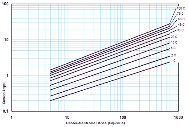
Graph equivalent to Figure 5-2 of the IPC-2152 standard
Other initial characteristics of this “universal table” are that it is generated for a copper thickness of 3 oz and on a polyamide substrate with a thickness of 70 mils (1.77 mm).
From this generic table, the standard establishes several other auxiliary tables with correction factors for the “universal” values based on different factors:
• Adjustment according to the base copper thickness: correction factors are generated for thicknesses of 0.5 oz, 1 oz, and 2 oz (3 oz is the initial value).
• Adjustment according to the plane closest to the trace that generates the heat. This plane has the greatest influence on heat dissipation, since it is the main dissipative surface, and correction factors are generated for planes at separations of 5, 20, and 40 mils.
• Adjustment according to the type of insulating material, consisting of an additional factor for PCBs made of FR4 material.
• Adjustment according to the total thickness of the PCB, with multiplication factors for thicknesses of 38 and 59 mils (70 mils is the initial value).
The various graphs and their correction factors allow us to calculate with reasonable accuracy the temperature increase the PCB will experience above ambient temperature.
If we add to this resulting temperature the safety margin we wish to establish in our project, we will obtain the minimum Tg temperature of the material with which we must manufacture our PCB.
Heat Generated by Discrete Components
In some cases, a discrete component may be operating within its own safe operating range, and at the same time the temperature its casing reaches is considerably higher than the Tg value of the PCB material (Author's note: this author can attest to having seen how a CMOS transistor melted the tin of its solder joints while maintaining stable operation and not being destroyed... although the same could not be said of the PCB where it was mounted).
This is the most common use case: excess heat. To address this problem, the approach known as thermal Ohm's law has traditionally been used. This approach equates the power dissipated by the component (W) to the current (A) in a conventional series resistor circuit. The excess heat to be absorbed (°C) is "dissipated" across the various thermal resistances (Rth in °C/W), just as the voltage (V) is distributed in our "virtual" circuit proportionally to the electrical resistances (Ohms).
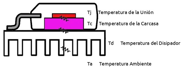
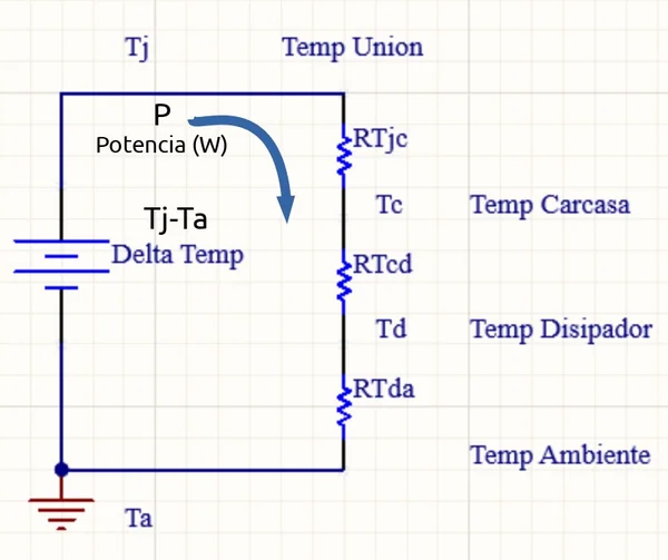
The development of this basic method is widely known, and it's easy to find information about it by searching online for the terms "thermal Ohm's law in PCBs." A thermal circuit that is no longer so easy to solve is the one shown in the attached figure, reminiscent of the complicated basic electronics exercises from my student days:

This case will not be explored in detail here, as we want this article to reach as many people as possible. However, the various thermal resistances between the different conductive planes involved, the thermal paths to the bottom layer, and the other thermal resistances already established in the basic example are clearly visible. The diagram represents the different paths and mechanisms of heat propagation within the PCB.
In any case, we can provide practical recommendations drawn from technical literature to achieve good thermal design (although these will never be able to improve upon modern simulation programs):
• On a double-sided PCB with solid copper, no heatsink, and natural air convection (no fan), the minimum area required to dissipate 1 W of
power for a 40 °C temperature increase is 15.3 cm². We are not referring to the copper thickness here since heat dissipation is by convection, not conduction. However, certain conditions are assumed: that air circulates freely on both sides of the PCB (the PCB is not inside a closed chassis), and also that the PCB has a good thermal design, optimally distributing heat from the source chip to the edges. The following points help optimize this second condition.
• The thicker the copper, the better the heat is conducted. A 2oz copper layer has 25% less thermal resistance than a 1oz layer (i.e., it improves heat dissipation by 25%).
• The copper plane through which heat propagates should be extended, and perpendicular cuts in the direction of heat propagation should be avoided.
• If available, place the heatsink along the path of least thermal resistance to the chip junction being cooled. A package with a bottom thermal gap has lower thermal resistance to the junction at this point, so a more favorable result is obtained if the heatsink is placed on the bottom face of the PCB.
• If there are multiple heat sources on the PCB, it is recommended to apply superposition. This involves solving for each heat source separately, calculating the temperature increase it causes at the locations of the other heat sources, and then summing all the individual contributions. This will give a good estimate of the temperature increase at each point.
Following these recommendations, we now list different effects on the final junction-to-ambient thermal resistance value θja for a chip already mounted on a circuit, with different PCB configurations:
• Increasing the number of layers improves overall heat dissipation: the improvement in thermal resistance between a 2-sided PCB and a 4-layer PCB with internal planes can reach up to 40% (the final θja decreases by 40%).
• The presence of separate planes on the TOP and BOTTOM sides, connected to the chip's support area or "dog bone," also improves its heat dissipation by up to 20%.
• The copper structure of these TOP and BOTTOM planes also influences the final thermal resistance: a copper coverage reduced to 50% of its ideal maximum surface area (a copper plane without discontinuities) worsens heat dissipation by approximately 3%.
• The solder mask on the TOP and BOTTOM planes improves heat dissipation by about 4-5% (the final θja decreases by that amount). The solder mask has better heat radiation than copper, although this may seem counterintuitive.
• Placing thermal vias in the "dog bone" region (beneath the chip package), along with their size, greatly improves heat dissipation, reducing the final θja. The recommended via diameter is 12–13 mils (0.30–0.33 mm), which can lower the final θja by 15–25%.
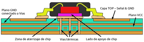
A through-hole via with a 0.3 mm (12 mil) diameter and 18 µm copper walls has a thermal resistance of 261 °C/W. The recommendation here is to place as many of these vias as possible—the number matters a lot—forming an array with 1 mm spacing on the exposed thermal pad.
• Factors with little effect on the total θja set:
✔ The location of the vias in the "dog bone" landing region.
✔ The location of the vias in the surrounding region, outside the dog bone region.
✔ Component package construction in the support area.
✔ Bonding wire materials (internal to the chip).
• Important factors:
✔ Chip size and landing surface size matter; larger is better.
✔ The percentage of PCB surface covered with solder mask is also important: the higher the percentage, the better. The total resistance θja is not significantly affected if the reduction from the maximum possible (100% of the PCB covered with solder mask) is less than 50% of the surface area (the deterioration of θja is less than 5%). However, when the coverage drops below this level, the thermal behavior deteriorates considerably (up to 35% if the solder mask coverage falls to 5% of the surface area).
Taking all these considerations into account, we could summarize them as a set of recommendations for optimized PCB design from a thermal point of view:
• Use the largest possible PCB surfaces with the thickest copper layers possible (at least four sides, 3”x3”, and 2oz/1oz/1oz/2oz thicknesses).
• Use thermal vias in the grounding area of the components to be cooled, connecting the top GND, inner GND, and bottom GND layers.
• Place thermal vias near the periphery of the exposed pads if the maximum number of vias cannot be placed across the entire surface.
• Create a ground plane as large as the PCB topology allows, especially near the package to be cooled, on the top, bottom, and middle layers.
• Connect the GND plane to the bottom ground pad of the “thermal” IC packages.
• Connect pins belonging to the same connection on each chip package, such as GND, PVIN, and POUT. This will maximize the copper area right next to the packages.
• Make the connection traces as long as possible since they serve to conduct heat to the outside of the chips to be cooled.
Heat generated by the PCB traces
To characterize the heating experienced by a PCB due to the current flowing through the conductive traces, the best normative reference is the IPC-2152 standard.
PCB construction
conditions
Using the graphs included in this standard, the temperature increase relative to ambient temperature is calculated, thus determining the final circuit temperature. This value must not exceed the critical Tg value of our PCB material.
Assuming the PCB under analysis or design has an area greater than 3x3 in² (a square with sides of 76.2 mm), the "universal chart" of the standard is used as the starting point. If the PCB surface area is smaller, the "conservative chart" is used.
These graphs directly show the cross-sectional area of a copper trace for a given current flow and expected temperature rise. As previously mentioned, these graphs are generated under specific operating conditions. Therefore, correction factors must be applied to adjust the results to the actual specifications of our circuit:
• A correction is applied for differences in copper size (the original graph was obtained for traces 3 oz thick).
• An additional correction is applied based on the presence and area of conductive planes near the trace, as these contribute significantly to heat dissipation. The original graph was obtained without adjacent planes.
• Another adjustment must also be applied based on the final total thickness of the PCB.
The universal graph is obtained for a total thickness of 70 mils (1.778 mm).
• If the PCB is constructed with FR-4 material instead of polyimide, another additional correction factor must also be applied.
All these corrective factors are tabulated in the standard, and through them, we can adjust the cross-sectional area of the conductor that produces the expected temperature increase in our PCB.
It's worth noting here that the graphs in the standard are based on the assumption that the traces being analyzed are separated by a distance greater than 1 inch (25.4 mm), which is often impractical. If the traces are closer together, their temperature will increase. To account for this effect, the combined current of all the traces should be used.
As an example, we summarize the design process of a heater implemented in practice on the internal traces of a 6-layer PCB. The traces that perform the heater function are located on layers L3 and L4, both surrounded by power and ground planes on L2 and L5, respectively. The PCB is constructed from FR-4 material, with a trace thickness of 0.5 oz on all internal layers. Since the PCB area is larger than 3x3", we can use the universal chart and apply the various correction factors.
The total PCB thickness is 61 mils (1.55 mm), with the two internal cores measuring 0.55 mm (21.65 mils) thick. There is also a 0.108 mm gap between them (achieved through a 4.28 mil thick layer of 2116 prepreg). The stackup details are shown in the following figure.
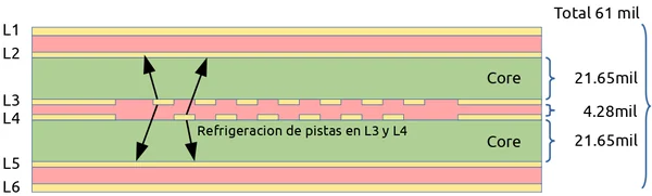
Each track forming part of the heater in L3 and L4 has a plane close to 21.65 mils, and another plane on the opposite side farther away at 25.94 mils (21.65 + 4.28). This results in double cooling for each of the radiant track layers in our heater. Considering these two effects separately, we will apply the IPC standard to calculate the individual effect of each plane close to the radiant tracks. Then, using superposition, we will calculate the total thermal resistance of the "parallel" equivalent of both thermal resistances. The effect is identical for the two thermal track layers L3 and L4.
As a starting point, we want the heater to increase the temperature of the PCB by about 15 °C, with a current available according to the design for it of 9 A.
Using the equivalent circuit approach for thermal resistances, which we presented in the previous section, since the generated heat has two simultaneous paths through which to dissipate, the effect generated by the two planes corresponds to the existence of two approximately equal thermal resistances in parallel. We know that the final resistance of two resistors connected in parallel is less than the smaller of the two, and that if they are equal, the result is half their value. Applying this concept to the temperature dynamics, in practice this means assuming that the PCB will cool approximately "twice as well" as if it only had one plane. Therefore, we will perform our calculations for each individual plane considering a desired individual temperature increase of 30 °C, assuming that the final temperature will be approximately the result of dividing the increase by two, obtaining the desired 15 °C.
From here, we use the IPC standard tables assuming that there is only one cooling plane instead of two, and we will assume, as we have said, an initial temperature increase of 30 °C.
Below, we provide an example of one of the iterations performed during the calculations.
Including the known variables without including any compensation, in the universal table we obtain the initial value of the copper cross-sectional area (Ac) of 299.7 mil², which is equivalent to a trace width (W) of 76.8 mils for 3oz thick traces, as contemplated by the universal table.
Ac = 299.7 mil², W = 76.8 mil @ 3oz, Temperature increase of 30 °C
We now include the following compensation factors:
• 1/2 oz traces instead of 3 oz: multiplier by 0.858 according to the copper thickness compensation table. Ac = 257.3 mils²
• Total circuit thickness of 61 mils instead of 70 mils: multiplier by 1.084 using the thickness table. Ac = 279 mils²
• Having a 1/2 oz plane at a separation of 21.65 mils from the traces: multiplier by 0.53, according to the plane proximity table. Ac = 147.5 mils²
• Having a plane acting as a heat sink with an area greater than 3x3 in²: multiplier by 0.95. Ac = 140.4 mils²
• We use FR-4 material instead of Polyimide: according to the material table, we apply a multiplier of 1.02. Ac = 143.2 thousand², W = 209.11 thousand
We then performed the same exercise for our next heat sink, which is located 25.94 mils from the heating tracks. The resulting cross-sectional area and trace width are as follows: Ac = 146.37 mil², W = 213.73 mils
Now we must perform several iterations until we obtain the same area result in both cases. To do this, we slightly modify the
temperature increments considered in each case until we obtain the same track width. In our case, we obtain the equilibrium value for the following result:
Ac = 142.9 mil², W = 208.6 mil, which is obtained for starting values:
• Temperature increase of 31.36 °C, for a plane separation of 21.65 mils.
• Temperature increase of 32.20 °C, for a plane separation of 25.94 mils.
If we calculate the final temperature increase produced by these two thermal resistors in parallel, we obtain a result of 15.88 °C, a value that is close enough to the initial design value sought.
On the other hand, recalling the initial data from our example, we assumed that our radiator operated with a heating current of 9 A. In practice, we're not going to design a PCB with a single 1/2 oz thick trace per inch of space and 208.6 mils wide through which we'll pass that current. Instead, we'll consider the cumulative effect of traces within a 1-inch area, the separation established by the IPC-2152 standard to generate all the tables we've relied on during the design process.
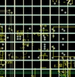 Mesh trace topology used, to consider the additive heating effect they produce, adding the current of all of them per surface inch.
For this purpose, we created a mesh along the two inner layers as shown in the figure, placing horizontal tracks on layer L3 and vertical tracks on L4.
This arrangement results in the track distribution shown in the following figures, with a total of 16 tracks located within an area of
1 in. on each side. We then divide the resulting total track width by the 16 tracks that will contribute to heating the area, obtaining a width per track of 208.6/16 = 13.04 mils (0.33 mm).
With this track width, a thickness of ½oz and a total length of 8.6m, the resulting resistance is 21.3 Ω, which, when connected to the output of a 12 V voltage regulator, produces a current of 0.562 A. Calculating the accumulated current flowing within our 1 in side space, we obtain the 9 A that we used in our initial calculations.
The distribution of this total track length within the PCB is done in compliance with the established separation to obtain 16 tracks/in., and the final results of the system's operation are shown in the following figures, obtained with a thermal camera.
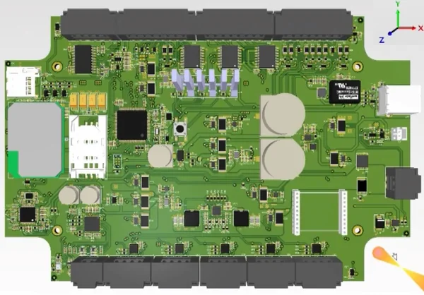
3D view of the PCB
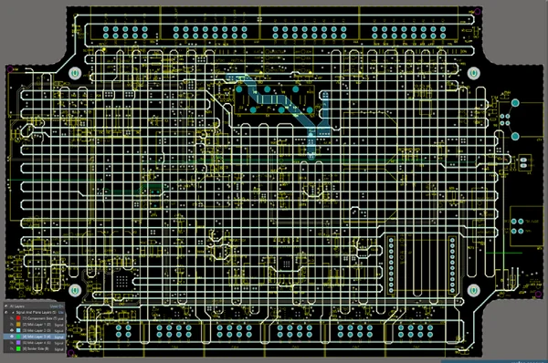
Detail of the tracks that function as a heater
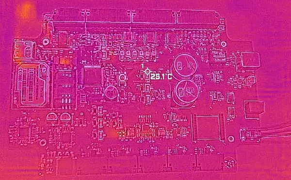
Thermal image at 25 °C
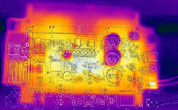
Thermal image at 31 °C

Thermal image at 35 °C

Thermal image at 40 °C
Conclusion
A review has been made of the considerations to take into account when
predicting the thermal behavior of a PCB, with special emphasis on the IPC-2152 standard, also showing an example of the use of said standard in the design of a heater
embedded within a PCB taking advantage of the heating induced by the passage of electric current through its tracks.
We hope that these design guidelines can serve as a starting point for your thermal design, and in any case, at NCAB we will be happy to help you with any
technical questions you may have to confidently tackle the thermal design of your PCB.
Author: By: Juan Luis Tébar García, NCAB Group http://www.ncabgroup.com/