Introduction
In applications such as electromagnetic (EM) flow meters and biopotential measurements, small differential signals are in series with much larger differential offsets. These offsets typically limit the gain that the circuit can support in the front-end design, which in turn impacts the overall dynamic range. Gain limitation is even more difficult when using lower supply voltages, for example, in battery-powered signal chains. One solution to this large differential offset problem is to use an AC-coupled measurement signal chain. A typical AC-coupled signal chain would include a low-gain instrumentation amplifier, followed by a high-pass filter and additional gain stages (see "Amplifying AC Signals with Large DC Offsets for Low-Power Designs"). In most applications, it is preferable to obtain as much gain as possible in the first stage, as this helps to improve the referred noise at input (RTI) of the subsequent gain stages in the signal chain. This article will help you design and implement an in-amp instrumentation amplifier architecture that allows for high gain and AC coupling, all in a single stage. The design will include the AD8237, a zero-drift, micropower instrumentation amplifier with a wide differential and common-mode input range. Other examples of in-amp architectures include the AD8420. The main advantages of such an in-amp current feedback amplifier are:
► Low power consumption.
► No diamond plot limitations as with other typical architectures like in-amps composed of two or three operational amplifiers (op amps).
► Good gain drift performance can be achieved through external resistor matching.
► High CMRR can be achieved without relying on resistor matching.
► High impedance reference pin.

Figure 1. AC coupled signal conditioning circuit with indirect current mode architecture.

The circuit in Figure 1 provides the general scheme in which the AD8237 indirect-mode amplifier is selected. However, to achieve high gain and AC coupling in a single stage, it is necessary to implement an integrator circuit in a feedback loop with the AD8237. This solution allows for higher gain than instrumentation amplifier solutions composed of two or three op amps, which cancel the offset once the gain is applied. In the proposed architecture, offset correction occurs before the gain phase, allowing the internal amplifier to have high gain. Both architectures are presented in the appendix. The ADA4505 operational amplifier is used in the feedback loop as the integrator circuit. The output of the AD8237 is sensed by the integrator input and drives the AD8237's reference pin to force the AD8237's output to VMID, which is set to the ADA4505's + input. Although the integrator provides a low-pass filter function, in this situation, due to its use in the feedback loop, the overall circuit will have a high-pass filter transfer function. Thanks to this behavior, it will not only ultimately block any DC deviation before the gain is reached, allowing for a greater gain increase than other solutions, but it is also even more useful with low supply voltages and large deviations, since the margin with which one can work is limited. The integrator also forces the AD8237 output to a chosen voltage via a reference pin. In fact, the integrator is forcing the reference pin relative to the AD8237's FB pin to be equal and opposite to the differential voltage of the inputs.

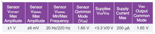
Table 1. Key design specifications for the circuit in Figure 1

Example Design Specifications
For low-power applications, a single power supply is typically available, usually between 1.8 V and 3.6 V. The design options for the circuit shown in Figure 1 depend on the amplitude and frequency range of the input signal and the offset. Table 1 lists example design specifications for the circuit in Figure 1.
The design options for this circuit were implemented using a low-bandwidth mode for the AD8237, which allows for gain flexibility and improved stability.

Design Description:
The circuit in Figure 1 consists of the AD8237, a rail-to-rail micropower instrumentation amplifier, and the ADA4505, a zero-input crossover distortion operational amplifier. Both can be powered from a minimum 3.3 V supply, VDD.
This circuit can supply a voltage, VOUT, representing the amplification of the AC signal, VSIGNAL, presented at the input while eliminating any DC offset voltage, VOFFSET. A voltage, VMID, is generated to adjust both the positive input of the ADA4505 and the common-mode output of the AD8237's gain stage to half the supply voltage. VMID is generated with a voltage divider (R1, R2) and buffered with another ADA4505. The AD8237 is in an MSOP (mini small outline package) and the ADA4505 in a WLCSP (compact wafer-level chip scale package).

Design Considerations
1. The positive input of the ADA4505-2 (1/2), VMID, will set the value of VREF (the AD8237's Ref pin) and, consequently, the output, VOUT. To ensure maximum output swing between the two supply channels, the optimal value for most instrumentation amplifiers is found at half the supply voltage (+VDD/2) due to the common-mode input voltage versus the output range, or diamond diagram. A diamond diagram tool will be presented in the design simulations section to assist with this task.
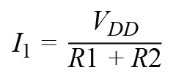
2. When considering the total supply current of the circuit, the choice of resistor values ​​R1 and R2 is also important. The resistor choice is a compromise between noise and power dissipation. In the case of this circuit, it is better to choose larger resistor values ​​to minimize the additional supply current. The additional supply current added for this resistor divider would be:

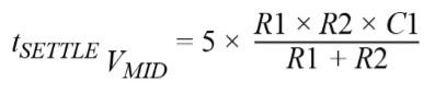
► In the case of the resistor divider (R1, R2), an additional capacitor C1 can be added to limit the noise band as well as reduce any 50 Hz/60 Hz or other interference on VDD. The larger the capacitor, the better the noise filtering; however, the VMID will take longer to stabilize upon power-up. The estimated time it takes to stabilize within 1% is:

3. When choosing the values ​​of the passive components (resistors and capacitors), tolerances must be taken into account. In the case of the resistor divider (R1, R2), the target value of VMID may shift, which would affect the output oscillation ranges (VOUT) of the AD8237 and the ADA4505.
Based on the circuit in Figure 1, the transfer function will have two cutoff frequencies resulting from a high-pass filter from the ADA4505 integrator in feedback and a low-pass filter response due to the bandwidth of the AD8237. Some gain error may be introduced, which is related to the cutoff frequency of the integrator (ADA4505) in combination with the bandwidth of the AD8237. Therefore, it is important that the high-pass and low-pass cutoff frequencies remain within a certain range. Depending on how close the cutoff frequencies are to each other, the percentage of gain error could change.
4. If the application requires the use of high-impedance sensors, buffers such as the ADA4505 can be used upstream of the AD8237 inputs to provide higher input impedance and lower input bias current, since a buffer will convert a high-impedance input to a low-impedance output. The AD8237's input bias current is 1 nA maximum over the temperature range.

Design Procedure
1. Voltage Divider to Adjust VMID:
Using section 2 of Design Considerations, for the circuit in Figure 1, the values ​​of the peripheral components are set to R1 = R2 = 1 MΩ to keep the supply current contribution around 1 µA.

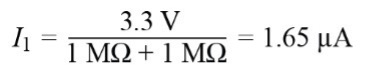
Output of the resistor divider before the ADA4505:

Assuming the tolerance for R1 and R2 is 5% and taking into account the offset of the ADA4505:

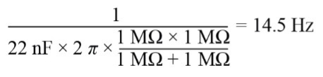
To eliminate AC power supply interference and resistor noise, adjust C1 so that the cutoff frequency is at least lower than the minimum VSIGNAL frequency of 20 Hz.

Please note that the capacitor value may be higher if necessary to further limit noise.

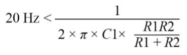
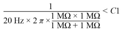
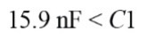
In this case, C1 is set to 22 nF, which provides a frequency of:

2. Instrumentation Amplifier (AD8237) Gain Value VSIGNAL:
Consider that the output range of EM flow sensors is typically a peak-to-peak signal amplitude ranging from ±75 µV to ±6 mV. For the circuit in Figure 1, the peak-to-peak signal amplitude range will be set to VSIGNAL = 6 mV peak at a frequency of 30 Hz.
Next, consider the output swing range limits of the AD8237 to the power supply channels. These values ​​can be found in the "Output Swing" datasheet. We will use the RL = 10 kΩ swing case at +25 °C to be conservative:

For a 3.3V power supply:

Since the output is fully differential, the output will oscillate with respect to VMID and will, in the worst case:

For positive input signals (VMIDMAX = 1.732 V):

For negative input signals (VMIDMAX = 1.568 V):

Now, to adjust the gain, sum the total of the expected differential input signals and use the smaller of the positive and negative swing ranges to set the maximum swing range:

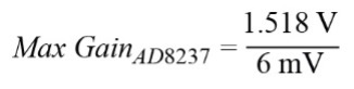
Considering the limits of the output voltage range, the gain of the AD8237 must be less than 253. To allow for DC/other errors, the gain value for the circuit in Figure 1 must be lower than the maximum possible value. There is also a trade-off between gain and settling time: the higher the gain, the slower the filter's time constant. Because of these considerations, the gain of the AD8237 is set to 101.
Note the benefit of the design considerations in Step 1 in terms of maximizing the swing value.
From the datasheet, the associated formula for the gain is:

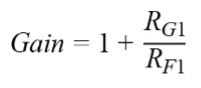
The AD8237 datasheet provides suggested resistor values ​​for gain selection. For a selected gain of 101, these resistor values ​​should be RF1 = 1 kΩ and RG1 = 100 kΩ.
3. Input Amplifier Bandwidth (AD8237):
From the datasheet, the cutoff frequency value is

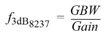
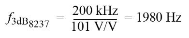
If the design specification requires a certain minimum attenuation for the maximum signal frequency, this can be easily checked for a given filter cutoff frequency.

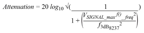
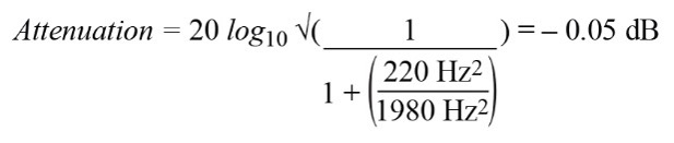
4. Adjusting the High-Pass Filter Cutoff Frequency:
A high-value high-pass filter cutoff frequency set by the integrator may get too close to the low-pass filter cutoff frequency set by the AD8237 bandwidth, as explained in the Design Considerations section. This will introduce some gain error relative to the previously set gain.
Assuming a tolerance of ±5% for R3 and C3, the fastest time constant should be less than the minimum V_SIGNAL.

The resistor R3 will have a constant value of 1 MΩ to minimize the current through this resistor to the operational amplifier.

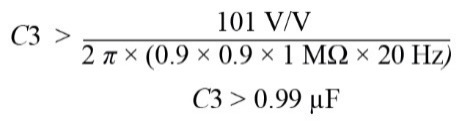
Taking the closest standard capacitor value to have approximately a cutoff frequency of 20 Hz, let's set C3 = 1.5 µF, so the updated cutoff frequency is:

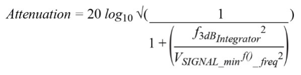
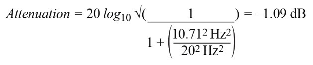
If the design specification requires a certain minimum attenuation for the minimum signal frequency, this can be easily verified for a given filter cutoff frequency. See an example of this circuit:

5. Offset Voltage:
Both the VOFFSET and VCM signals have limitations.
As expected, the DC offset can be higher than what is typically found in most applications. In this situation, the voltage value must be VOFFSET ≤ ± VMID. If the DC offset is greater than this limit, the VREF voltage value falls outside the ADA4505's supply voltage range. The equation related to the reference pin is: VREF = VMID - VOFFSET. VOFFSET will be set to 1 V.
As for the common-mode voltage, it is directly related to the VOFFSET value since VCM must be within the specified range.

If these limitations are not verified, the AD8237's input values ​​will be above or below the supply ranges. The VCM will be set to 1.65 V.

Design Simulations
To check the common-mode input range versus the output voltage or diamond diagram of an instrumentation amplifier, you will need to provide the supply voltage +VDD, reference voltage, gain, common-mode swing, and differential input swing. The Analog Devices Instrumentation Amplifier Diamond Diagram tool helps you see if the input swing is within the component's operating range. Note that the output swing used for the tool uses worst-case load conditions (smallest resistive load), so if you design within the tool's limits, there will be additional margin for larger resistive loads. Looking at the results in Figure 2, the purple contour is the usable range of the AD8237 for the supply voltage, output swing, input common-mode range, and component reference voltage. The red contour shows how much of this range is being used for the given common-mode and differential input swing. The goal is to keep the red contour within the purple contour. If certain conditions are not met, the tool will display the error and offer recommendations. It is important to note that implementing the integrator circuit in the feedback loop is not possible with this interface. However, one workaround is to configure the input signal of the diamond diagram as if the VOFFSET and VCM voltages of the circuit (in Figure 1) were added. This eliminates the range (0.65 V to 2.65 V) as a DC offset, and no gain is achieved. It also shows that the common-mode voltage could be higher, as there is still some headroom for the output to oscillate. To better understand what is happening inside the instrumentation amplifier, the Internal Circuitry tab displays the voltages of the internal nodes.

Figure 2. An example of the AD8237 plotting tool.

LTspice® is an excellent simulation tool for verifying the design procedure calculations performed earlier, including other specifications of interest such as noise performance in the signal band of interest. The LTspice schematic is shown in Figure 3. The first simulation (Figure 4 and Figure 5) is a transient simulation with a 1 V DC offset and a ±6 mV input signal at 30 Hz. Figure 4 shows the signal at different stages of the circuit. Figure 5 is an enlarged version of Figure 4 after the circuit has settled and the integrator capacitor has charged to its final value. The blue curve is the integrator output or reference voltage pin of the AD8237. The red curve is the designed VMID value at VDD/2, and the green curve is the final 30 Hz output signal, VOUT.

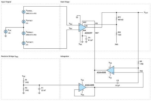Figure 3. LTspice Schematic

Table 2 shows a comparison of the design objective versus the simulation results for the transient simulation. For the maximum and minimum values ​​of VOUT, the expected values ​​are derived from: VOUT = VMID ± VSIGNAL × 101, which in our case gives us expected values ​​of 2.256 V and 1.044 V. The expected value of VREF is equal to VMID - VOFFSET, which in our case gives us an expected value of 0.65 V. As for VMID, we calculated it to be the average supply voltage, which in our case is 1.65 V.

Figure 4. Transient simulation results.

The results obtained in the transient analysis, compared to expectations, are quite similar in terms of output voltage. However, it takes 17 seconds for the simulation to settle and for the output to reach its final value, due to the large integrating capacitor and the large DC offset implemented. This settling time is because the simulation starts at time 0 s, and the capacitor needs time to charge to its final value.

Table 2. Design objective versus simulation Transient analysis

Design Target Parameter Simulation

The simulation in Figure 6 shows the frequency response of the circuit in Figure 3 with a DC offset of 1 V and an input signal of ±6 mV at 30 Hz. Cursors 1 and 2 in Figure 6 were set to the -3 dB point for the high-pass and low-pass filters, respectively. Table 3 shows a comparison between the design objectives and the simulation results.

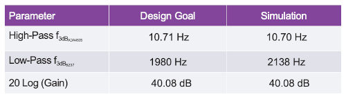Table 3 Design objective versus simulation AC analysis

Design Target Parameter Simulation

 The following simulation in Figure 7 shows the voltage noise density versus frequency RTI for the circuit in Figure 3. This is done by dividing the output noise by the total gain of the solution (101). For the bandpass filter function, we need to choose the integration frequency range to calculate the total noise.
For the upper frequency, we will use the sensor's maximum frequency value set earlier, which is 220 Hz. For the lower frequency, we will also use the sensor's minimum frequency value set at 20 Hz. In this situation, the resulting noise will be from the integration from 20 Hz to 220 Hz.

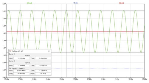
Figure 5. Extended transient simulation results.

In reality, the measured noise will be higher due to the bandpass filter's cutoff frequencies. The LTspice simulation results assume a post-processing "brick wall" filter to have a sharp roll-off at 20 Hz and 220 Hz.

The command line in LTspice is then set to .noise V(VOUT) V1 dec 100 20 220. Next, hold down the control key and left-click on the waveform name (V(ONOISE)/101). The RMS noise can be easily converted to peak-to-peak noise using the equation:


A quick noise check of the AD8237 and ADA4505 determined that the AD8237 is the dominant noise source.

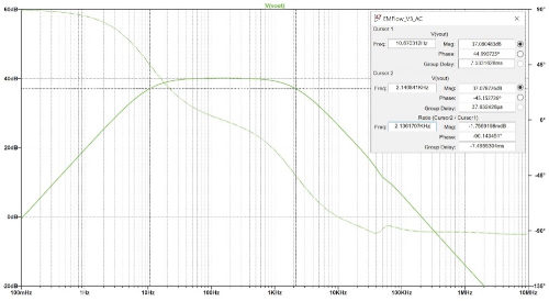Figure 6. AC simulation results.

Figure 7. Total noise integrated into the equivalent noise bandwidth.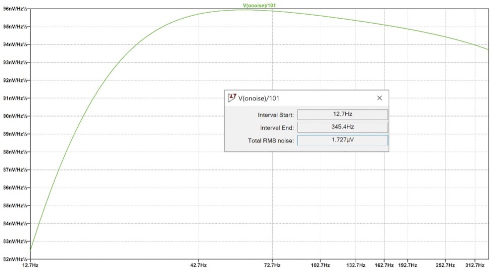

Measured Results:
To highlight the above results, hardware testing is possible, as both the AD8237 and ADA4505 offer breadboards. Each component can be soldered using the breadboard schematics. When using both breadboards simultaneously, it may be necessary to cut a trace on the AD8237 board to connect the VMID voltage to the RG resistors.
For clarity, component values ​​were established and taken from the design procedure section, as with the design simulation. To simulate the EM flow meters or biopotential measurement sensors, different measuring equipment was used, such as a voltage calibrator and an arbitrary waveform generator.

For this test, the input signals were set with a DC offset, VOFFSET, of 1 V, a common-mode voltage of 1.65 V, and an input signal, VSIGNAL, of ±6 mV at 30 Hz.
Observing the results shown in Figure 8, the output voltage performance VOUT (yellow curve) has a small deviation from the expected values, but is still in line with expectations.

Table 4 shows a summary of the design objectives versus the measured results.

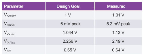Table 4. Design objectives versus measured results

The differences between the design objective and the simulation results can have various origins.
► The resistors used had a 5% error tolerance, meaning the VMID value could have shifted.
► The test bench configuration may have limitations that could lead to minor deviations, as shown in the measured simulations, VOFFSET and VSIGNAL.

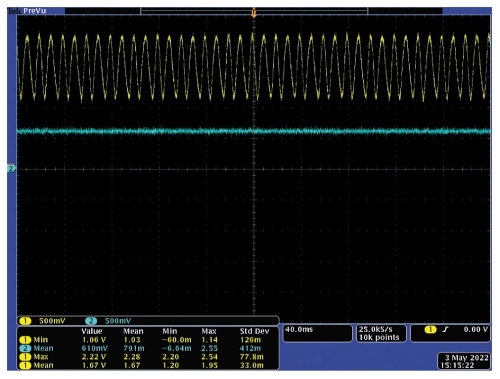Figure 8. Screenshot of an oscilloscope with the yellow curve corresponding to VOUT and the blue curve VREF.

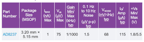
Design devices

Conclusion:
A common requirement when capturing signals from sensors such as EM flow sensors in field transmitters or electrodes in biopotential applications is that the signal of interest is often based on much larger DC offsets. To facilitate the extraction of relevant information from these sensors, one solution is to implement an AC-coupled measurement signal chain. The goal is to eliminate DC offsets while amplifying the AC signals. The AD8237 instrumentation amplifier provides the gain, and the AC is coupled in a single stage by incorporating an integrator circuit in the feedback loop. By eliminating DC offset at the input stage, this circuit allows maximum signal gain to be applied directly to the input of the measurement signal chain, minimizing noise referred to the input of the overall measurement solution.

References
LTspice
LTspice is a high-performance SPICE III simulator, schematic capture and waveform viewer with enhancements and models to facilitate the simulation of switching, linear and signal chain regulator circuits.

Diamond Plot Tool for Instrumentation Amplifiers
The Diamond Plot Tool is a web application that generates a configuration-specific output voltage range versus input common-mode voltage plot, also known as a diamond plot, for ADI instrumentation amplifiers.

Appendix
Figure 9. Instrumentation amplifier in indirect current mode Architecture of the AD8237 instrumentation amplifier in indirect current mode.

Figures 9 and 10 show the current-indirect mode instrumentation amplifier and the three-op-amp instrumentation. The current-indirect mode instrumentation amplifier allows for higher gain than instrumentation amplifier solutions composed of two or three op-amps, which cancel the offset once the gain is applied. In the proposed architecture, offset correction occurs before the gain stage, allowing the instrumentation amplifier to have a high gain. Both architectures are described below.
In Figure 9, the current-indirect mode instrumentation amplifier is based on a single-stage configuration. The input voltages are applied to the first cell, GM1, while cell GM2 is in the feedback loop. The internal integrator, Amplifier A, forces a replica of VIN1 onto VIN2. The integrator is used to drive the reference pin, which is prior to the gain stage. The gain is adjusted by the external resistors RFB and RG and is equal to:

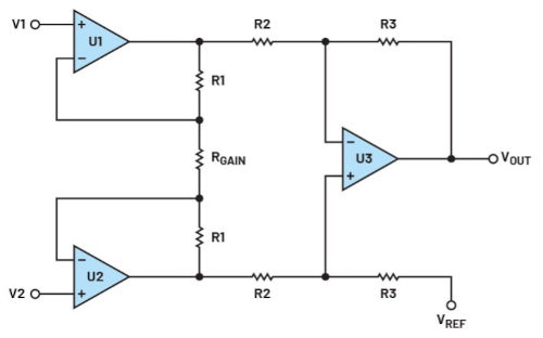Figure 10. Three operational amplifier instrumentation amplifiers. Three operational amplifier instrumentation amplifiers.

The three-op-amp architecture in Figure 10 is based on a two-stage configuration. The first two operational amplifiers, U1 and U2, the RGAIN resistor, and resistors R2 and R1 form non-inverting amplifiers and are considered the input stage. It provides unity common-mode gain, and the differential gain is adjusted by the RGAIN resistor and is equal to:

The last operational amplifier, U3, and resistors R3 form a differential amplifier that constitutes the output stage of the instrumentation amplifier. It provides unity gain in differential mode and common-mode rejection. The reference injection point for this architecture is located in the second stage after the first gain stage.

Acknowledgments
Key Consultants:
David Plourde, CI Design Engineer, Scientific Instruments Group (SCI)
Aine McCarthy, Senior Systems Applications Engineer, Automotive Group
Tim Green, Senior Analog Applications Engineer, Scientific Instruments Group (SCI)

Author: Marie-Eve Carre, Systems Applications Engineer, Analog Devices.
About the author:
Marie-Eve Carre holds a Master's degree in Electronic Engineering from the CPE School of Engineering in Lyon, France. Marie-Eve first joined Analog Devices in 2020 as an applications engineering cooperative before returning to France to complete her Master's degree. She rejoined ADI in 2022 and currently supports the Precision Signal Chains applications group with a focus on low-power signal chains.