


This is largely because these systems are more integrated into relatively small SoCs, FPGAs, or ASICs. These customer-specific application processors and their functions are at the heart of modern electronics, from very simple in-house developments to the latest IoT applications or the ubiquitous electronics we use every day.
Many developers working on custom embedded designs rely on their oscilloscopes to debug and visualize many different types of problems. Affordable oscilloscopes have been able to analyze basic timing and noise issues, signal quality, and data problems for several years. With many older oscilloscope features, such as using digital channels in MSO (mixed-signal analysis), serial decoding, and signal search and recording, this device is the most important tool for basic troubleshooting in any engineer's workplace. However, when it comes to certain challenges, such as jitter analysis or investigating signal distortions, the limitations of a conventional oscilloscope are quickly reached. This requires expanded analysis functions, which are usually outside the budget of the average engineer.
High-end oscilloscopes have long offered options for extended analysis and measurement functions, such as jitter analysis, which is essential given the complexity of modern design development. Rigol's UltraVision II platform combines multiple custom ASICs with FPGAs into a highly integrated, reliable, and affordable test platform based on an advanced analysis and debugging concept. The MSO8000 series oscilloscope (header image) is Rigol's most comprehensive embedded design tool, capable of characterizing signals up to 2 GHz and analyzing complex signal integrity, distortion, and timing issues.
In summary, the MSO8000 series offers the most comprehensive analysis capabilities, the deepest memory, and the highest sampling rate in its class. The MSO8000's features are designed for embedded design and fault analysis to accelerate the review and debugging of modern testing challenges. The functions for performing complex signal analysis quickly and easily are described in detail below.

Characterizing Jitter Behavior:
The accuracy of a signal cycle is crucial for digital data transmission, especially at high data rates. Even the most subtle changes in clock frequency influence error rates and data throughput. However, these time-based errors cannot be visualized simply with a traditional oscilloscope as was previously used at common serial communication speeds.
The MSO8000 series' jitter analysis function provides the solution. Utilizing high sampling rates and deep memory, the oscilloscope compares timing changes across thousands of clock transitions. This allows for the visualization of timing fluctuations below 100 picoseconds, and these changes can be tracked over extended periods.
One of the keys to visualizing jitter is the Time Interval Error (TIE). The TIE is defined as the time difference between the ideal clock edge and the actually measured clock edge. There are two measurement methods that can be used to analyze errors when measuring the TIE. One is the TIE trend plot. This graph shows the cumulative error of the TIE values over time. This trend visualization is a valuable analysis tool because it highlights the periodic causes of fluctuation. Figure 2 shows a high-speed clock signal (channel 1, yellow) and the TIE fluctuation trend (purple).

The unit of the vertical axis shown here for the TIE trend is 10 nanoseconds/DIV. The trend shows that the TIE jitter behaves periodically. This means that a periodic signal or event affects the clock frequency. The TIE trend can be measured more accurately using the cursor (see Figure 3). With the cursor, you can easily measure the signal period and calculate the frequency (1/DX). Direct measurements can also be taken on the TIE trend. The period of the TIE trend is an important indication of the source of jitter problems.
In addition to the TIE trend, you can also calculate the distribution of TIE values. The shape and standard deviation of the TIE values are important for determining the cause. Visualizing the signal histogram is suitable for this (see Figure 4). 
It is important to have a proper understanding of the nature of TIE values and trends, and how to interpret the distribution. As already described, the TIE is calculated as a periodically accumulated change in the interfering signal. This means that the TIE trend resembles the integral of the interfering signal. Therefore, a square wave change in period can be derived from the TIE trend in Figure 4. In this example, it can be seen that the period of the clock signal increases linearly (increasing trend) and then decreases linearly again (decreasing trend). This linear increase also shows that the clock period of the signal is stable, but it must be greater than the expected optimal clock period. The same is true for the linear decrease, where the period must also have a stable value and is less than the expected period. Therefore, the period changes between two stable values that are once above and once below the expected period. The frequency measurement in the trend shows that the cause of the fluctuation is a 10 kHz square wave signal. The histogram display shows that the fluctuation appears to be constant because the TIE distribution is distributed uniformly and symmetrically over these values.

For the measured circuit, nearby signal sources were measured and the 10 kHz interference signal was determined (see Figure 5, blue curve).
Jitter can be caused by various factors, including problems with the PLLs, current fluctuations in the circuit, or interference emissions. The following examples will focus more on using histograms to measure jitter, as they illustrate the changes resulting from jitter correction.
Since both sinusoidal and triangular interference waves have a sinusoidal integral to the cause of jitter, it is insufficient to draw conclusions about the interference source based solely on the trend. The histogram and its standard deviation are additional tools for more accurately identifying the interference signal. For example, the histogram in Figure 6 shows a bimodal distribution of TIE values with a sinusoidal TIE trend.
The histogram statistics measure a standard deviation (sigma value) of approximately 3.2 nanoseconds. Since the mean value of this trend is close to zero, the standard deviation in the histogram can also be approximated as the RMS value of the trend signal (see RMS value measurement, bottom left). The graphical representation of the histogram can help visually represent potential skewness, for example, when the signal deviates slowly and then corrects quickly.
Figure 7 shows a good example of an asymmetric fluctuation distribution that still appears almost sinusoidal in the TIE fluctuation trend. This distribution facilitates the identification of the process that may be causing the variability.
Jitter analysis is important because it concerns data integrity and, ultimately, errors that cost system time or bandwidth. Therefore, simply analyzing the timing variation is insufficient; how the data is presented to the user is equally important. The MSO8000 offers several clock recovery methods for measuring jitter. A serial data stream can use an explicit clock or be processed according to a defined clock frequency. Alternatively, the data stream could also use a PLL circuit to determine the period.
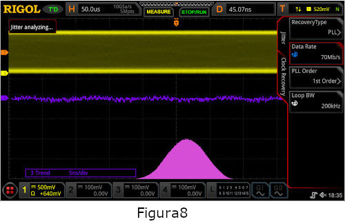
The measurements described above were performed with a constant clock setting. In contrast, Figure 8 shows a jitter measurement of the same signal from Figure 7, performed on the MSO8000 using a first-order PLL recovery method with a loop bandwidth of 200 kHz. With this dynamic clock recovery, the jitter behavior is significantly improved, and the bimodal fluctuations in the histogram are no longer present.
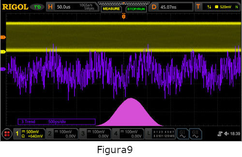
A vertical zoom of the trend is now useful for analyzing finer jitter fluctuations (in Figure 9, 500 psec./DIV). Periodic jitter is still visible here, but it has been significantly reduced and will likely no longer affect potential bit errors.
As soon as all jitter occurrences have been analyzed and eliminated, the trend can be further reduced (below 500 ps/DIV) to analyze noise behavior (see Figure 10). The MSO8000 also allows a direct statistical table view of TIE values, as well as a comparison of one period cycle to the next (cycle-to-cycle) or a comparison of the positive/negative pulse to the next (+/- width to +/- width). Once all system jitter has been successfully addressed, noise sources below 500 picoseconds per division can be displayed, as shown in Figure 10. The MSO8000 oscilloscope also allows a direct statistical table view of TIE values, as well as cycle-to-cycle values and values calculated from the positive and negative widths.
 Taken together, this new jitter analysis tool allows for careful visualization and analysis of jitter problems in key serial communication links that are far beyond the capabilities of a typical mid-range oscilloscope.
Signal Quality Diagram and Eye Diagram:
Jitter behavior is just one of the characteristics that contribute to overall signal quality. The goal of all forms of analysis related to signal quality is to reduce data errors in transmitter-to-receiver communication. Errors are often caused by timing and jitter issues. However, problems can also arise from insufficient bandwidth, an incorrect ground connection, increased noise behavior, or inadequate impedance matching, all of which negatively affect how the receiver interprets a bit. The best method for visualizing the overall data signal quality is to display the Eye Diagram—a pattern of the transmitted data signal. Traditionally, these measurement methods are found on high-power, high-priced oscilloscopes. Real-time Eye Diagram display is an excellent way to validate and debug serial data links where throughput and a low bit error rate are critical to system performance.
The Eye Diagram analyzes the overlapping, aligned data lines of the signal and synchronizes these bit sequences with the restored clock. The clock recovery options already described, which can be selected for jitter measurement, can also be used for Eye Diagram analysis. The Eye Diagram is created by overlaying each bit sequence. A density diagram is then created from thousands of bit sequences. This will create a pattern, which can be seen in Figure 11. This pattern is called the Eye Pattern or Eye Diagram because the shape in the center resembles an open eye that closes at a point on each side. The goal is to have an open eye and thus correctly interpret the bit states (0 or 1) in the middle of the eye.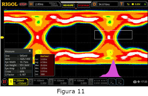
This advanced analysis method allows for the verification of cables and connectors. Furthermore, the impact on signal quality during the design process can be identified through undesirable effects such as crosstalk or other emissions.
For example, the Eye Diagram in Figure 11 shows some potential problems. Depending on the threshold value set on the MSO8000, the instrument calculates the width and height of the eye. Due to the less pronounced edges of the eye, you can see that this signal has a limited bandwidth, which can be problematic. The quality can be analytically assessed by ensuring that the eye level, eye width, and signal rise time are equal to or better than the values indicated in the data sheet. Frequency uncertainties with respect to the recovery clock also occur in the same measurement. This can be seen by the fact that the histogram curve does not show a Gaussian distribution, as might be expected with good signal performance. Furthermore, the eye exhibits some noise behavior; that is, the amplitude fluctuates during transmission, and the eye closes vertically.
Once the problem causing the frequency fluctuation has been identified and the interference has been eliminated, the eye will open again (see Figure 12).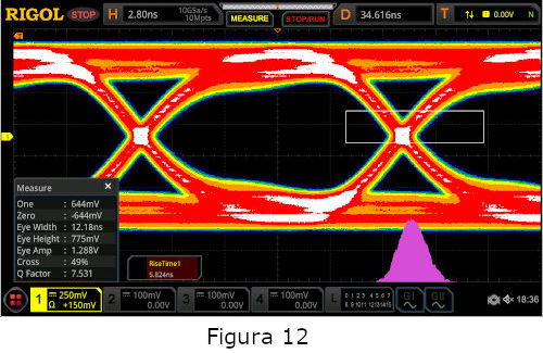
The histogram graphic display now shows that the remaining frequency fluctuation is at least symmetrical. This improvement is also noticeable in a wider eye. Once the nearby noise source is identified and eliminated, both the height and width of the eyes improve (see Figure 13), and the signal becomes more accurate.
 With this measurement, it is now even more clearly visible that the signal has a bandwidth problem, as the edge slope can be better analyzed here with the narrower eyelines. It can also be seen here that there are still different amplitude values during data transmission, which still slightly narrow the eyeline.
Finally, in Figure 14, an improved bandwidth can be seen after the transmitter circuit was replaced with an improved version. The histogram distribution shows that some of the outliers in the signal fluctuation no longer occur. The improved bandwidth is clearly evident in the improved slope and a fully open vertical eyeline.
Abstract:
Fault analysis of digital data signals in embedded designs is a critical requirement in modern electronics. Modern, high-performance digital oscilloscopes expand the analytical capabilities available to engineers for everyday needs. Rigol's UltraVision-II technology and the MSO8000 series oscilloscopes complement these tools with the option of Jitter and Eye diagram analysis. This comprehensive signal quality analysis is also attractively priced and easy to use. Jitter and Eye diagram analysis on the MSO8000 greatly simplifies the visualization and analysis of overall signal quality in serial data connections and the troubleshooting of issues related to clocking, noise behavior, and bandwidth. With new analysis functions, as well as a memory depth of 500 Mpts and a high sampling rate (10 GSa/s), which are based on the UltraVision II platform, Rigol's MSO8000 series offers a complete solution for current development in this area.
 Author: Author: Boris Adlung, RIGOL Technologies, Gilching