

 Radar has advanced a great deal since the late 19th century and has evolved into a set of technologies that currently supports a wide range of applications.
These range from the simple, affordable, and compact continuous-wave (CW) radar, used by law enforcement to catch speeding drivers, to complex active phased array (APAS) antennas used in land-based, naval, and airborne radar systems. A typical APAS or active electronically oriented radar (AESA) consists of hundreds or thousands of transmitter/receiver (T/R) modules, made possible by high-performance solid-state devices.  As radar technologies reach higher frequencies and wider bandwidths, new applications previously unimaginable have emerged. Low-cost, ultra-wideband, non-ionizing microwave imaging provides distinct information from existing imaging techniques and offers promising applications in the medical and healthcare fields. Submillimeter-resolution radar gesture recognition offers consumers new ways to interact with devices. Radar technologies have also enabled autonomous driving and drones, with their autonomous capabilities and collision avoidance features. The THz band, with its unique spectral properties regarding chemical and biological content, attracts both scientific and non-scientific communities with potential applications in imaging, sensing, and detection. As radar offers increasingly diverse applications, we would like to briefly review the timeless principles of radar.
Operating Principle:
The essence of radar is its ability to gather physical information about one or more targets: location, speed, direction, shape, identity, or simply their presence. This is achieved by processing reflected electromagnetic waves in the case of primary radars, or from a transmitted response in the case of secondary radars. In most implementations, the radar system generates a pulsed RF or microwave signal and directs it toward the target. The same antenna that transmitted the signal then receives it back.
The basic block diagram of a pulse radar system is shown in Figure 1. In this diagram, the main timer or pulse repetition frequency (PRF) generator is shown as the central block of the system. The PRF generator plays a crucial role in synchronizing all the components of the radar system through connections with the pulse modulator, the duplexer or transmit/receive switch, and the display processor. In addition, the connections to the receiver would provide filtering for front-end protection or time-based gain control, such as sensitivity time control (STC).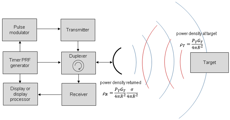
Figure 1. Example block diagram for a pulse radar system.
Explanation of the radar equation:
The radar equation describes the most important performance variables of a radar and provides the basis for understanding the measures taken to ensure optimal performance. The equation can be presented in many different forms. Equation 1 shows one form of the radar equation that gives the maximum range of a radar in meters. To better understand the stated equation and the assumptions used, it is best for readers to review Derivation 2. 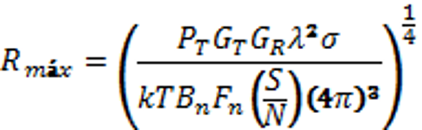
(1)
Where:
R = maximum distance in meters
PT = transmitted power in watts
GT = transmitting antenna gain
GR = receiving antenna gain
λ = radar signal wavelength in meters
α = radar cross-section (RCS) of the target in square meters
k = Boltzmann constant
T = ambient temperature in Kelvin
Bn = receiver noise bandwidth in hertz
Fn = noise figure
S/N = minimum required signal-to-noise ratio
The derivation begins with the analysis of a simple spherical scattering propagation model for an isotropic radiator (or point source antenna). Since radar systems employ directional antennas to concentrate the radiated energy on the target, the antenna gain is defined as the ratio of the power directed toward the target to the power of an ideal isotropic antenna. The equation reflects the directional antenna gain with GT and GR for transmitting and receiving, respectively. If the same antenna is used for both transmitting and receiving, the equation can be simplified by replacing both terms with G.
Part of the transmitted power density reaching the target will be reflected in various directions, while some of the energy will be re-radiated back to the radar system. The amount of this incident power density that is re-radiated to the radar is a function of the radar cross-section (RCS or α) of the target. The RCS (α) is expressed in area units and is a measure of the size of the target as seen by the radar.
The radar antenna will intercept a portion of this signal reflected by the target. This signal power will be equal to the return power density at the antenna multiplied by the effective area of the antenna. The main factors limiting the receiver are noise and the resulting signal-to-noise ratio (SNR).
The noise power (theoretical limit) at the receiver input is described as Johnson noise or thermal noise. It is a consequence of the random motion of electrons and is proportional to the temperature. The noise power available at the receiver output will always be higher than the Johnson noise. This is due to the extra noise generated within the receiver. Consequently, Equation 1 accounts for the noise generated within the receiver by multiplying the Johnson noise power by the noise factor F<sub>n</sub> and the receiver gain.
Equation 1 describes the maximum range of our radar target based on the transmitter power, antenna gain, target RCS, system noise figure, and minimum signal-to-noise ratio. In reality, this is a simplified model of system performance. Many other factors will also affect this performance, including modifications to the assumptions used to derive this equation. Two other elements that should be considered are system losses and pulse integration, which may be applied during signal processing. System losses will be found in both the transmit (LT) and receive (LR).
In a classic pulse radar application, we could assume that multiple pulses would be received from a given target for each position of the radar antenna (since the radar antenna beamwidth is greater than zero, we can assume that the radar will remain on each target for a period of time) and, therefore, could be integrated to improve the performance of the radar system. Since this integration might not be ideal, an integration efficiency term Ei(n) based on the number of integrated pulses will be used to describe the improvement in integration. Including these terms, the radar equation becomes: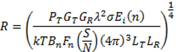 (2)
(2)
Where: E i (n) = integration efficiency factor LT = transmission path losses LR = reception path losses For multi-antenna radars, the radar range will increase proportionally to the number of elements, provided all elements offer identical performance. Conclusions on the radar equation The signal power at the radar receiver is directly proportional to the transmitted power, the antenna gain (or aperture size), and the radar cross-section (RCS); that is, the degree to which a target reflects the radar signal. And perhaps more importantly, it is inversely proportional to the fourth power of the distance to the target. In view of the large attenuation that occurs as the signal travels to and from the target, high power is highly desirable. However, achieving high power is difficult due to practical problems such as heat, voltage collapse, dynamic power requirements, system size, and cost.
In the next article, we will discuss the characteristics, compression techniques, and measurement of pulsed radar signals.
References:
1. https://atap.google.com/soli/
2. http://literature.cdn.keysight.com/litweb/pdf/5992-1386EN.pdf?id=2715324
Author:
Giovanni D'Amore
Marketing Brand Manager - EMEAI
RF & Microwave Products
Keysight Technologies
Radar has advanced considerably since the late 19th century, evolving into a suite of technologies that now supports a wide range of applications. These range from the simple, affordable, and compact continuous-wave (CW) radar, used by law enforcement to catch speeding drivers, to complex active phased array (AESA) radar systems used in land-based, naval, and airborne radar applications. A typical AESA radar consists of hundreds or thousands of transmitter/receiver (T/R) modules, made possible by high-performance solid-state devices.
As radar technologies reach higher frequencies and wider bandwidths, new applications previously unimaginable have emerged. Low-cost, non-ionizing, ultra-wideband microwave imaging provides distinct information from existing imaging techniques and offers promising applications in the medical and healthcare fields. Submillimeter-resolution radar gesture recognition offers consumers new ways to interact with devicesbothautonomy and collision avoidance. The THz band, with its unique spectral properties regarding chemical and biological content, attracts both scientific and non-scientific communities with potential applications in imaging, sensing, and detection. As radar offers increasingly diverse applications, we would like to briefly review the timeless principles of radar.
Operating principle
The essence of radar is its ability to gather physical information about one or more targets: location, speed, direction, shape, identity, or simply their presence. This is achieved by processing reflected electromagnetic waves in the case of primary radars, or from a transmitted response in the case of secondary radars. In most implementations, the radar system generates a pulsed RF or microwave signal and directs it toward the target. The same antenna that transmitted the signal then receives it back.
The basic block diagram of a pulse radar system is shown in Figure 1. In this diagram, the main timer, or pulse repetition frequency (PRF) generator, is shown as the central block of the system. The PRF generator plays a crucial role in synchronizing all the radar system components through connections to the pulse modulator, the duplexer or transmit/receive switch, and the display processor. Additionally, connections to the receiver provide filtering for front-end or timed gain control, such as sensitivity time control (STC).

Figure 1. Example of a block diagram for a pulse radar system
Explanation of the radar equation
The radar equation describes the most important performance variables of a radar and provides the basis for understanding the measures taken to ensure optimal performance. The equation can be presented in many different forms. Equation 1 shows one form of the radar equation that gives the maximum range of a radar in meters. To better understand the equation and the assumptions used, it is best for readers to review the derivation2.
 (1)
(1)
Where:
 = maximum distance in meters
 = transmitted power in watts
 = transmitting antenna gain
 = receiving antenna gain
 = wavelength of the radar signal in meters
 = Radar cross-section (RCS) of the target in square meters
 = Boltzmann constant
 = ambient temperature in Kelvin
 = receiver noise bandwidth in hertz
 = noise figure
 = minimum signal-to-noise ratio required
The derivation begins with the analysis of a simple spherical scatter propagation model for an isotropic radiator (or point source antenna). Since radar systems employ directional antennas to concentrate radiated energy on the target, the antenna gain is defined as the ratio of the power directed toward the target to the power of an ideal isotropic antenna. The equation reflects the antenna's directive gain, with and for transmitting and receiving, respectively. If the same antenna is used for both transmitting and receiving, the equation can be simplified by replacing both terms with  .
.
Part of the transmitted power density reaching the target will be reflected in various directions, while some of the energy will be re-radiated back to the radar system. The amount of this incident power density that is re-radiated to the radar is a function of the radar cross-section (RCS ) of the target. The RCSis expressed in area units and is a measure of the size of the target as seen by the radar.
The radar antenna will intercept a portion of the signal reflected by the target. This signal strength will be equal to the return power density at the antenna multiplied by the effective area of the antenna. The main factors limiting the receiver are noise and theresulting signal-to-noise ratio (SNR).
The noise power (theoretical limit) at the receiver input is described as Johnson noise or thermal noise. It is a consequence of the random motion of electrons and is proportional to the temperature. The noise power available at the receiver output will always be higher than the Johnson noise. This is due to the additional noise generated within the receiver. Therefore, Equation 1 accounts for the noise generated within the receiver by multiplying the Johnson noise power by the noise factor and the receiver gain.
Equation 1 describes the maximum range of our radar target based on the transmitter power, antenna gain, target RCS, system noise figure, and minimum signal-to-noise ratio. In reality, this is a simplified model of system performance. Many other factors will also affect this performance, including modifications to the assumptions used to derive this equation. Two other elements that should be considered are system losses and pulse integration, which may be applied during signal processing. System losses will be found in both the transmit  and receive
  .
.
In a classic pulse radar application, we could assume that multiple pulses would be received from a given target for each position of the radar antenna (since the radar antenna's beamwidth is greater than zero, we can assume that the radar will remain on each target for a period of time) and could therefore be integrated to improve the radar system's performance. Since this integration might not be ideal, an integration efficiency term  based on the number of integrated pulses will be used to describe the improvement in integration. Including these terms, the radar equation becomes:
 (2)
(2)
Where:
= integration efficiency factor
= losses in the transmission path
= losses in the receiving route
For multi-antenna radars, the radar range will increase proportionally to the number of elements, provided that all elements offer identical performance.
Conclusions on the radar equation
The signal strength at the radar receiver is directly proportional to the transmitted power, the antenna gain (or aperture size), and the radar cross-section (RCS); that is, the degree to which a target reflects the radar signal. Perhaps more importantly, it is inversely proportional to the fourth power of the distance to the target. Given the significant attenuation that occurs as the signal travels to and from the target, high power is highly desirable. However, achieving high power is challenging due to practical issues such as heat, voltage collapse, dynamic power requirements, system size, and cost.
In the next article, we will discuss the characteristics, compression techniques, and measurement of the pulsed radar signal.
References:
1. https://atap.google.com/soli/
2. http://literature.cdn.keysight.com/litweb/pdf/5992-1386EN.pdf?id=2715324