

Modern beamforming integrated circuits (BFICs) typically have multiple parallel on-chip RF paths with independently controllable gain and phase. Common BFIC configurations have two or more of these on-chip RF paths connected to pins located on the same edge and/or corner of the IC package. Figure 1 shows a 4-input, 4-output BFIC with all four inputs on the same edge of the IC package and all four outputs on opposite edges. This device architecture is used in ADAR3000/ADAR3001/ADAR3006/ADAR3007 of Ku- and Ka-band beamforming integrated circuits. The BFIC must also support all the digital, power, and other miscellaneous pins required for its operation.
The relatively close pin spacing in the BFIC is a consequence of the large number of RF inputs and outputs and their associated signal-to-ground configuration. Routing multiple high-precision RF lines from these closely spaced pins to various devices, connectors, or other printed circuit boards (PCBs) presents a challenge. Low transmission line impedance accuracy and poor impedance transitions (e.g., at the transition between two boards) cause signal reflections. This reduces the RF power delivered to the load and decreases gain. Lower system gain and reduced output power degrade the effective isotropic radiated power (EIRP) of the transmitters. Sufficiently large signal reflections can also cause instability, especially if the circuit design is susceptible to reflected power from its load.
This article discusses how to design and fabricate high-precision RF PCB transmission lines and connector transitions with excellent return loss that route signals to and from the PCB via transmission lines connecting to high-count RF input and output BFICs. Although focused on BFIC and phased-array applications, the material is equally applicable to any high-frequency circuit design where good impedance matching is important. Multiple design techniques will be presented, but the important topic of design for manufacturing will also be addressed. Note that this article provides dimensions primarily in thousandths of an inch (1000 thousandths of an inch equals 1 inch). To convert from thousandths of an inch to millimeters, multiply by 0.0254.
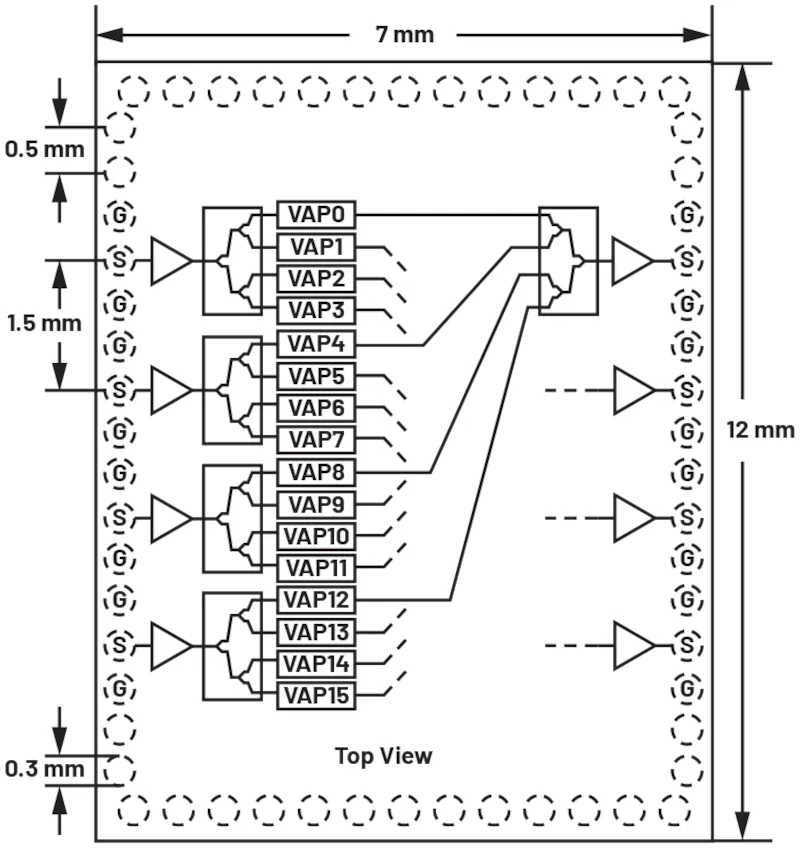
Figure 1. Anatomical block diagram of a 4-input, 4-output, 16-channel BFIC chip in a BGA package; the outline dimensions are not to scale with the pitch between balls and the diameter of the balls.
Fabrication of Various Transmission Line Topologies:
PCB manufacturers support several popular RF transmission line topologies, including microstrip, grounded coplanar waveguide (GCPW), stripline, and the less popular buried GCPW (BGCPW), which resembles a hybrid between GCPW and stripline. Although microstrip is relatively easy to fabricate, it is less popular for operation above 6 GHz due to its higher trace loss and poor mode suppression.<sup>1</sup> GCPW, BGCPW, and stripline perform better above 6 GHz due to their lower radiation loss and better mode suppression. Buried line topologies improve isolation but are more difficult to fabricate and require vias for connection. These vias are typically blind to minimize parasitic inductance, resulting in a higher board cost.
Figure 2 shows a cross-section of GCPW, buried GCPW, and a band line, as well as the important geometries that determine the nominal line impedance. These are the line width (W1/W2/W3), the lateral distance from the line edge to the adjacent ground plane (G1/G2/G3), the thickness of the dielectric materials (T1/T2), and the relative permittivity of the dielectric materials (εR1/εR2). Figure 2 does not show the thickness of the copper used for the lines or the required grounding. The copper thickness must be considered, but it is a secondary effect. The required grounding will be discussed in Part 2. The choice of topology depends on the acceptable trace loss, the frequency, the required line-to-line isolation, the available space, and the dielectric thickness of the PCB material.
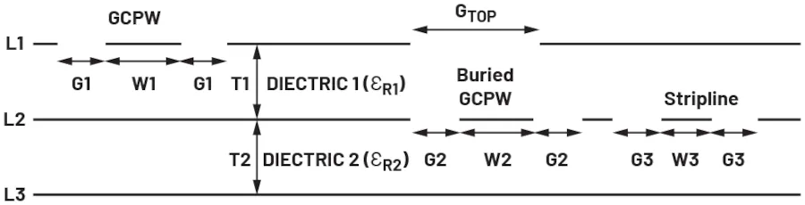
Figure 2. Cross-section of the GCPW, buried GCPW and line-of-band topologies.
Effects of Manufacturing Tolerances on Line Impedance:
The quality of RF line topologies is affected by manufacturing tolerances. Choosing optimal line geometries to minimize these effects is crucial for achieving an accurate 50 Ω line impedance. Figure 3 shows a time-domain reflectometry (TDR) plot of a 3-thousandths-of-an-inch-wide band line that was designed for 50 Ω but measured at approximately 60 Ω. An error of no more than ±10% (45 Ω to 55 Ω) was desired to achieve a return loss of 20 dB or better.
Three important geometries to consider when designing the line are line width, lateral ground clearance, and dielectric thickness. Many PCB manufacturers offer minimum conductor widths as low as 3 thousandths of an inch (depending on the copper weight) with a tolerance of 1 to 2 thousandths of an inch.<sup>2-4</sup> Manufacturers typically provide only typical dielectric thickness figures, likely because the final thickness is determined by the PCB manufacturer during the board lamination process. The side clearance to ground can vary as a result of the ground plane not stopping where it should. Furthermore, the effective width of the side clearance changes if the line width varies.

Figure 3. TDR plot of a 3-thousandths-of-an-inch wide band line on layer 2 of a PCB.
In microstrip and band line topologies, variations in the side gap width should not affect the line impedance, as the side distance to ground is large by design. This causes all field lines to flow to the lower ground plane in the case of microstrip and to the upper and lower ground planes in the case of band line. However, GCPW is more affected by side gap tolerances. By design, the side distance between the gap and ground is relatively small, and most field lines flow to the side ground plane.
Figure 4 shows the line impedance 5 of a band-line design versus the line width deviation from the nominal value for multiple line widths. It also shows the impedance deviation that occurs when the dielectric is 5% thicker than the nominal value (assuming a band-line copper thickness of 0.7 mils and εR = 3.1). Ideally, the slope of all lines would be 0, and there would be no offset at the intersection between lines, indicating no manufacturing variations. Note that wider lines have a shallower slope, while narrower lines have a steeper slope. Therefore, in practice, when manufacturing variations exist, a wider nominal line width is preferable. Unfortunately, with a 5% increase in dielectric thickness, the impedance offset is approximately the same regardless of the nominal line widths. This means the manufacturer must meet the final pressed thickness requirements within a certain tolerance to achieve the desired line impedance tolerance. The focus is on increasing the dielectric thickness (as opposed to decreasing it) because it has been observed in many manufacturing batches of boards with different line topologies that the line impedance tends to be greater than or equal to the design target. This leads to the general rule of designing the line with a few ohms less than the target, especially when the width is thin (less than 5 thousandths of an inch). However, with this approach, it may be necessary to forgo the controlled impedance requirements that normally constrain the PCB manufacturer, depending on the impedance difference. If a thin line must be used due to other design considerations, it is critical to have a high degree of confidence in the chosen manufacturer. Trust can be gained organically by using a manufacturer's previous designs and/or intentionally by fabricating experimental boards with the chosen line topology, featuring multiple lines of varying widths that would result in a design impedance of approximately 50 Ω. Measurements would then need to be taken to determine which line width most closely approximated 50 Ω.

Figure 4. Impedance error (for 50 Ω) versus manufacturing tolerance for line widths of 3, 5, 7 and 10 thousandths of an inch over nominal dielectric thickness and +5%.
On-Board Connections: PCB Signal Input and Output.
The RF impedance discontinuities between the RF transmission lines and the RF connectors that move signals between PCBs are just as important as the precise line impedance discussed earlier. When transitioning between boards, there are two physical interconnection options:
1. Side-launch connectors that mount laterally to the edge of the PCB.
2. Vertical-launch connectors that mount vertically to the PCB.
Both types are available in SMA, SMP, SMPM, 2.92 mm, and 2.4 mm, to name a few standards.
The choice between side-launch and vertical-launch will largely depend on the form factor of the final equipment. If side-launch connectors are used, the interconnecting PCB will be mounted laterally. If the system is housed in a single metal chassis/heatsink, this arrangement may be the best option. If vertical-launch connectors are used, there is the possibility of stacking multiple boards in a sandwich configuration. This can result in a more compact form factor, but it may also necessitate air cooling, as individual boards are unlikely to have heatsinks. A combination of both connector types—one board with side-launch and the other with vertical-launch—will cause the two boards to connect orthogonally in a slot-like fashion.
Side-launch connectors versus vertical-launch connectors:
Side-launch connectors are widely used. However, they have some potential drawbacks stemming from their attachment to the board edge. Side-launch connectors typically require a longer trace, compared to vertical-launch connectors, from the device to the connector. This results in increased insertion loss, parasitic capacitance, and inductance. Side-launch connectors also require the PCB's upper ground plane (and preferably the lower ground plane) to extend to the board edge. Most PCB manufacturers can only guarantee a clearance of 0.2 mils between the ground plane edge and the board edge at connector locations when using standard edge milling/routing and etching back-off techniques. This manifests as an impedance discontinuity due to the lack of ground return in the 0.2 mil (or greater) space and degrades return loss. This discontinuity becomes more pronounced at higher frequencies.
Figure 5a shows a PCB edge connector transition with a large gap between the board edge and the ground plane, while Figure 5b shows a TDR plot illustrating the impedance peak produced by a large gap in the connector. At lower frequencies, the gap may not affect performance and could even be desirable, as it keeps the end of the fragile transmission line away from the milling cutter that is machining the board edge. A simple solution is to terminate the transmission line 0.2 millimeters before the ground plane edge, which is a sufficient distance to keep it away from the milling cutter (preventing damage) while still providing a good transition for the center pin of the connector. This technique is often used in high-frequency millimeter-wave applications.

Figure 5. (a) Top view of an edge connector transition with a large gap between the PCB edge and the top layer ground plane and (b) TDR graph of a poor transition due to poor edge routing creating a large gap (the second connector launch peak is due to less reflected energy).
There are a couple of options for mitigating the gap between the ground plane and the board edge. The first is to use an edge trim at the connector locations on the board edge. When done correctly, this effectively eliminates the gap entirely by applying a metallic ground trim to the vertical edge of the board. The edge trim connects to the existing top and bottom horizontal ground planes and can also connect to internal ground planes if desired. The edge trim should only be on the grounded portions of the edge, and therefore, there must be a gap between the trim at the connector locations where the transmission line is located. This is shown in Figure 6.

Figure 6. Cross-section of a PCB at the edge connector location showing proper edge overlay.
Edge overlay presents some drawbacks stemming from manufacturing quality. This can result in:
• A rounded cut from the circular milling cutter used to remove the overlay on the transmission line (it is desirable to keep the PCB edge flat).
• Inconsistent milling before edge overlay occurs, leading to transmission line length matching issues (it is very important to maintain the same length as the calibration traces).
• Overlay extending from the ground locations on the board edge and encroaching on the transmission line area. The worst case is that the overlay is continuous across the entire connector location, including where the transmission line is located, as shown in Figure 7. This can cause the transmission line to short to ground.
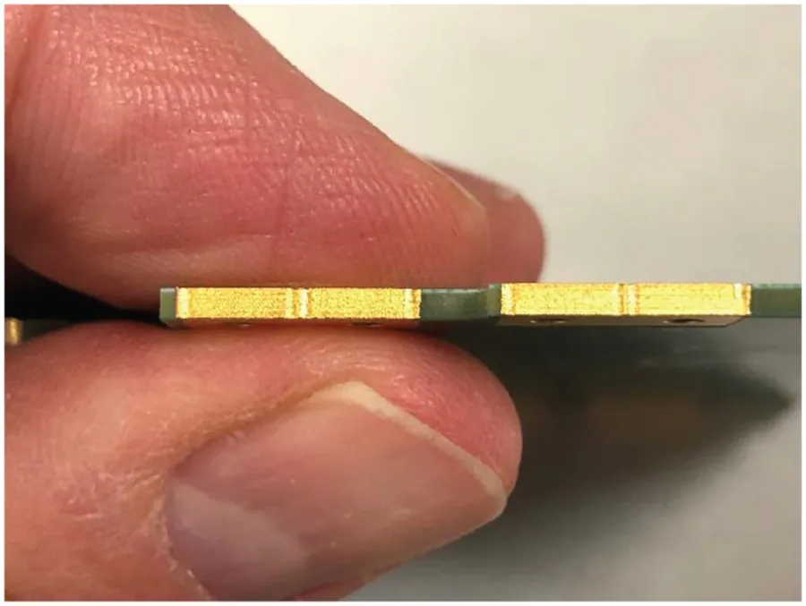
Figure 7. Example of edge covering encroaching from ground locations into the transmission line area (PCB side view).
The first two quality issues are undesirable and degrade PCB performance. However, they are not catastrophic. The third quality issue is catastrophic and renders the PCB unusable, requiring mechanical rework to remove the edge coating in the transmission line area. The only viable way to ensure high-quality edge coating is to mandate edge coating requirements in the PCB manufacturing notes. Depending on the stringency of these requirements, manufacturers may have to remake batches of PCBs. Or they may reject the job.
Laser edge milling is another option. Laser edge milling involves cutting the board with a laser. This can be done along the entire edge of the board, but it is only necessary at the connector locations, with mechanical milling of the remaining edge. Not all PCB manufacturers offer laser edge milling. Suppliers who do this typically guarantee only a margin of error of 1 mil, which is generally only achievable if the PCB is relatively thin. Some PCB manufacturers require the board to be less than 14 mils thick, while others can offer this accuracy on boards as thin as 40 mils. This is still relatively thin and raises the possibility of board warping, especially for larger boards, and is usually not thick enough for boards with a high layer count.
Edge coating and laser edge milling can increase cost, complexity, and manufacturing time. If the form factor of the final equipment allows the boards to be sandwiched together (rather than joined side-by-side), vertical-launch interconnects may be a viable option.
Vertical Launch Interconnects:
Because they are not attached to the edge of the board, vertical launch connectors are not susceptible to the edge routing problems described earlier. On simple single-device boards, the connectors can be placed close to the device under test, resulting in minimal insertion loss.
Furthermore, the transition to the board can be RF matched to minimize impedance discontinuity. Connector vendors, such as SVMicrowave, will create a custom footprint for a given line layout and stack. Figure 8 shows a footprint for an SVMicrowave vertical launch connector connecting to a band line layout. Four PCB layers with the via fencing are shown. The 0.30-thousandths-of-an-inch diameter gap in layer 3 (L3) is the fitting for the connector and is shown in Figure 8c.
One disadvantage of vertical launch connectors is that achieving good alignment between the connector and the printed circuit board footprint can be challenging. Ideally, the circular center pin of the connector should connect to its circular pad on the printed circuit board (PCB), and their centers should be aligned. However, when viewed from below as the connector is mounted on the 2D ground plane, some left-to-right and front-to-back movement may occur, which can cause the center pin to become misaligned with the PCB pad. Connectors intended for top-layer lines have a hole on the front that can be helpful for alignment, especially for left-to-right movement (these hole connectors have also been used successfully with band lines). The tolerance for the mounting hole size should be tight to minimize excessive connector movement. If precise alignment is required, as is the case for frequencies >35 GHz, Rosenberger offers connectors that are pitched at 45° to the board (as opposed to vertical 90° connectors) and can be manually aligned much more easily than vertical connectors. However, these 45° launch connectors are more expensive than their vertical and side-launch counterparts and require significantly more PCB space ( ).
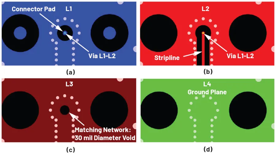
Figure 8. Custom vertical connector footprint design: (a) top ground in layer 1, (b) band line in layer 2, (c) a 30-thousandths-inch gap in layer 3 for adaptation, and (d) a solid ground plane in layer 4.
Conclusion:
The advent of high-frequency beamforming ICs and other high-frequency multichannel RF ICs is making PCB design more complex. When tackling these complex designs, PCB designers must anticipate potential manufacturing problems by avoiding the use of very thin RF traces and generally designing for a characteristic impedance slightly lower than the target value of 50 Ω. When designing board-to-board interconnects, top-launch or side-launch interconnects will most likely be chosen depending on the form factor of the final equipment. Top-launch interconnects are less susceptible to manufacturing constraints that can occur at the board edge.
The second part of this series of articles will discuss how transmission line isolation can affect the performance of high-frequency beamforming ICs, the isolation differences between transmission line topologies, and how to choose the best transmission line for a given application and BFIC geometry.
References
1 John Coonrod . “Comparison between Microstrips and Grounded Coplanar Waveguides” . Rogers Corporation.
2 “ PCB Manufacturing Tolerances ” . MADPCB.
3 “ Tolerances ”. AdvancedPCB.
4 “Tolerances”. Imagineering, Inc.
5 “ Stripline ”. Microwaves101.
About the author:
Joel Dobler is a senior product applications engineer in the Aerospace, Defense, and Communications Group, where he focuses on beamforming products but also supports vector modulators and programmable low-pass filters. He has worked for Analog Devices since 2006, supporting a wide range of RF products, including logarithmic and RMS detectors, digital and analog variable-gain amplifiers, mixers, and I/Q demodulators. He received his bachelor's degree in electrical engineering from Washington State University in 2005 and his master's degree in electrical engineering from Portland State University in 2007.