


Introduction
A variety of topologies can be considered for applications requiring the generation of a negative voltage channel, as illustrated in the article "The Art of Generating Negative Voltages."¹ However, if the absolute voltage at the input and/or output can exceed 24 V and the required output current can reach a few amperes, the charge pump and negative LDO regulator must be discarded due to their low current capacity, while the size of their magnetic components makes flyback and Ćuk converter solutions quite cumbersome. As a result, under these conditions, the buck-boost inverter offers the best compromise between high efficiency and small form factor.
However, to take advantage of these benefits, a thorough understanding of the operation of the buck-boost inverter topology under high-voltage conditions is necessary. Before going into detail, we will begin with a brief review of the buck-boost inverter topology. We will then compare the critical current paths of the buck-boost, buck, and boost inverter topologies.
The three basic non-isolated topologies:
The inverting buck-boost belongs to the three basic non-isolated switching topologies. All of these topologies consist of a control transistor (usually a MOSFET), a diode (which can be a Schottky diode or an active diode, the synchronous MOSFET), and a power inductor as an energy storage element. The common connection between these three elements is called the switching node. The position of the power inductor with respect to the switching node determines the topology.
If the inductor is placed between the switching node and the output, we obtain the DC-DC buck converter, which we will simply call buck in the rest of this article. If, on the other hand, the inductor is placed between the input and the switching node, we obtain the DC-DC boost converter, which we will call boost here. Finally, the DC-DC inverting buck-boost consists of placing the inductor between the switching node and ground (GND).
During each switching period, and even in continuous conduction mode (CCM), all three topologies include components and PCB traces that experience rapid current changes, resulting in the noisy transitions highlighted in Figure 1c, Figure 2c, and Figure 3c. By keeping the hot loop small, electromagnetic interference (EMI) radiated by the circuit can be reduced. It's worth noting that the hot loop is not necessarily a physical loop through which current flows. In fact, for the respective loops highlighted in Figure 1, Figure 2, and Figure 3, the abrupt current transitions do not occur in the same direction for the components and traces highlighted in red and blue that form the hot loop.
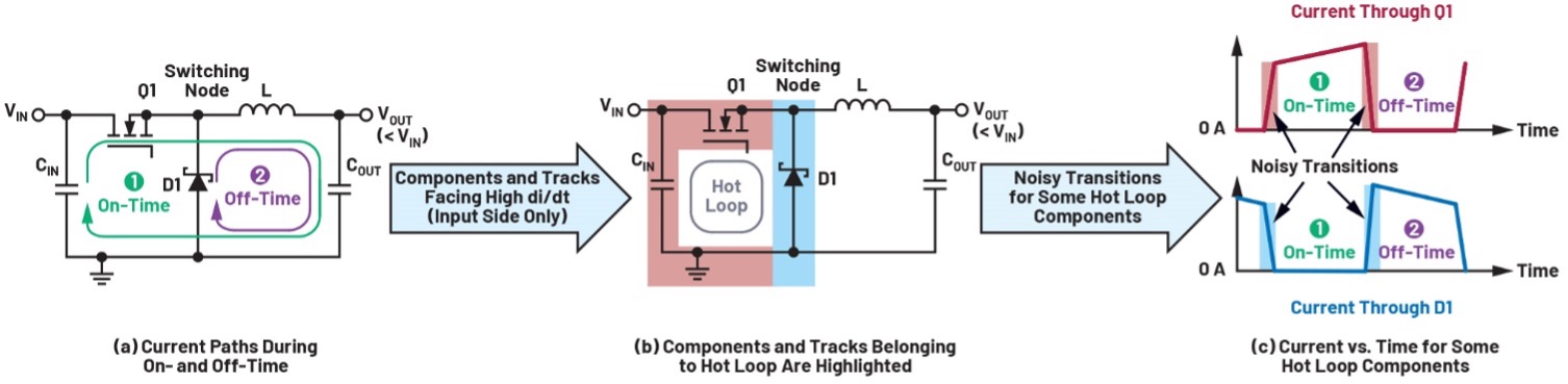 Figure 1. Components and traces belonging to the hot-loop converter operating in CCM.
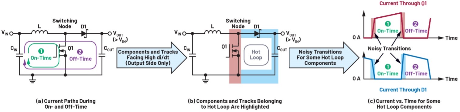
Figure 2. Components and tracks of the hot loop-boost converter operating in CCM.
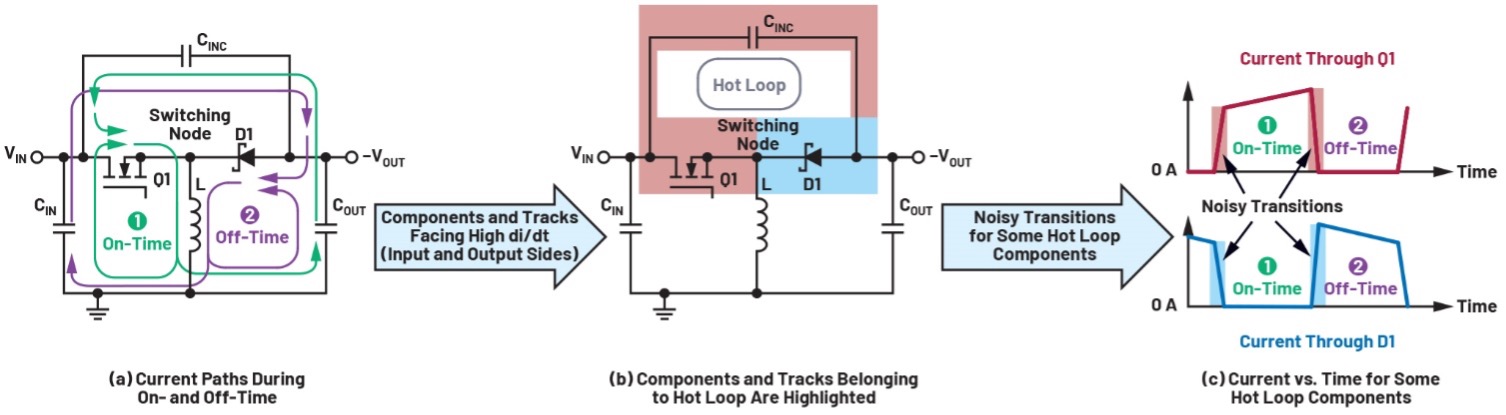
Figure 3. Components and traces of the hot-loop inverter buck-boost converter operating in CCM.
For the inverting buck-boost converter operating in CCM, as shown in Figure 3, the hot loop consists of CINC, Q1, and D1. Compared to the hot loop of buck and boost topologies, the hot loop of the inverting buck-boost contains components on both the input and output sides. Among these components, the reverse recovery of the diode (or body diode if a synchronous MOSFET is used) when the control MOSFET turns on generates the highest di/dt and EMI. Since careful design is needed to contain the radiated EMI from these two sides, the last thing desired is to create additional radiated EMI through excessive coil current ripple by underestimating the required inductance of the inverting buck-boost under high input and/or output voltage conditions. This risk exists for engineers who rely on their familiarity with the boost topology to size the inductance of their buck-boost inverter circuit, as we will now see by comparing both topologies.
Design considerations for Buck-Boost inverters with high voltages
Both the boost and buck-boost inverters can generate an absolute output voltage whose amplitude is greater than the input voltage. However, there are relevant differences between the two topologies, which can be highlighted using their respective duty cycles in CCM, provided in Equation 1 and Equation 2. Note that these are first-order approximations that do not account for effects such as voltage drops across Schottky diodes and power MOSFETs.

The first-order approximation for the variation of these duty cycles with respect to |VOUT| and with VIN = 12 V is represented on the left side of Figure 4. Furthermore, assuming in both cases a switching frequency (fSW) of 1 MHz and an inductance of 1 µH for the power coil, the variation of the coil current ripple with respect to VOUT.
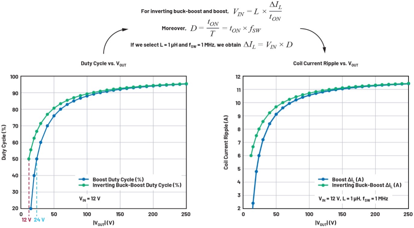
Figure 4. Duty Cycle. Duty cycle and coil current ripple versus |VOUT| at VIN = 12 V for inverting buck-boost and boost.
We observe in Figure 4 that the duty cycle of an inverting buck-boost will exceed 50% starting from a much lower |VOUT| than that of the boost: 12 V and 24 V, respectively. This can be understood by referring to Figure 5.
In the case of the boost, the inductor is located in the path between the input and the output. Therefore, the voltage across the power inductor (VL) is added to VIN to provide the necessary VOUT. However, in the case of the inverting buck-boost, VL is the only factor that contributes to the obtained output voltage. In that case, the power inductor must supply much more energy to the output, which explains why the duty cycle already reaches 50% for a much lower |VOUT|.
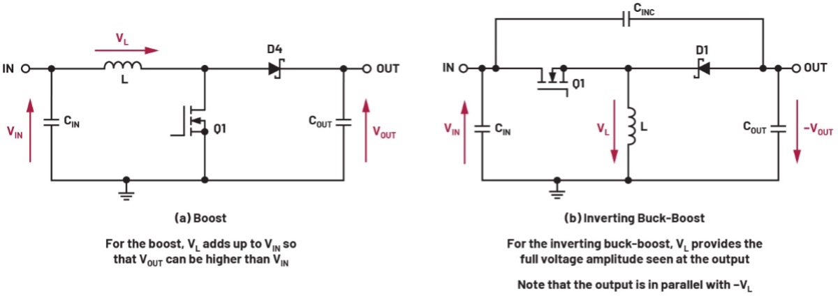
Figure 5. Impact of coil positioning on the output voltage.
We can rephrase this observation by stating that, as the ratio |VOUT|/VIN decreases, the duty cycle drops much more slowly for the buck-boost inverter than for the boost inverter. This is an important factor to consider during the design phase, and its impact can be better understood by referring to Figure 6, which again shows the first-order approximation of the coil duty cycle and ripple current, this time plotted against VIN.
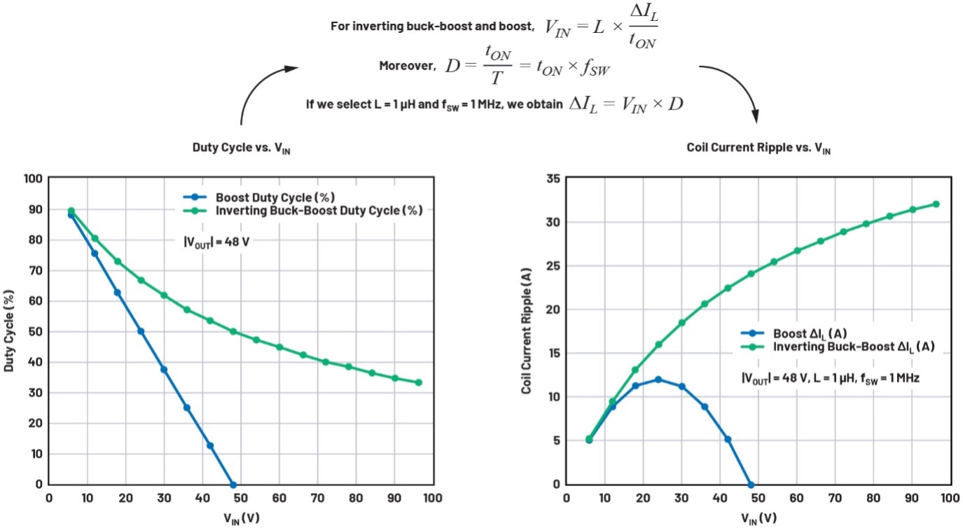
Figure 6. Duty Cycle and Inductor Current Ripple. Duty cycle and inductor current ripple versus VIN at |VOUT| = 48 V for inverting buck-boost and boost.
As shown in Figure 6, the inductor current ripple (ΔIL) is proportional to VIN and D. In the case of boost, as VIN becomes greater than half of VOUT, the duty cycle decreases faster than VIN increases, going from 50% at VIN = 24 V to a quarter of this value at VIN = 42 V for the blue curve on the left side of the graph in Figure 6. Consequently, ΔIL decreases rapidly for VIN above 24 V for boost in the right side of the graph in Figure 6.
However, for the inverting buck-boost, we already saw in Figure 4 that D decreases very slowly when |VOUT|/VIN decreases, or in other words, when VIN increases for a given |VOUT| fixed. This can be observed in the green curve on the left side of Figure 6, where the duty cycle only drops by 25% when VIN increases by 62.5% from 48 V to 78 V. Since the decrease in D does not compensate for the increase in VIN, the inductor current ripple increases significantly with VIN, as illustrated by the green curve on the right side of Figure 6. In general, the inductor current ripple is greater when VIN increases.
Overall, the greater inductor current ripple that the buck-boost inverter can face under high-voltage conditions compared to the boost inverter explains why the former topology requires higher inductor values if it operates at the same switching power (fSW). Let's apply this knowledge to a specific case using Figure 7, which is also based on first-order approximations.
Application with wide input voltage range and high output current
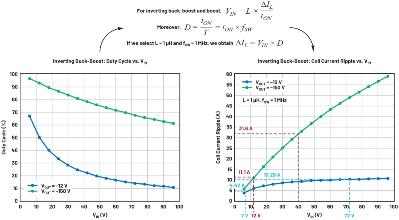
Figure 7. Duty Cycle. Duty cycle and coil current ripple versus VIN at VOUT = -12 V and -150 V for buck-boost inverter.
Application with wide input voltage range and high output current.
Let's consider an application with VIN = 7 V to 72 V and VOUT = -12 V at 5 A. Given the high output current, we opted for a synchronous controller (LTC3896) to achieve high efficiency.
Inductance Selection:
When operating the LTC3896 in CCM, it is recommended to keep ΔIL between 30% and 70% of IOUT,MAX, which is 5 A in our example. Consequently, we want to design for ΔIL between 1.5 A and 3.5 A across our entire input voltage range. Furthermore, staying within this recommended range of 30% to 70% of IOUT,MAX means that we can only allow a ratio of up to 2.33—that is, 70% divided by 30%—between the highest and lowest current ripple across our input voltage range. This is not a trivial task for a topology like the buck-boost inverter, where ΔIL varies significantly with VIN, as noted earlier.
Referring to Figure 7, when using fSW = 1 MHz and L = 1 µH, the coil current ripple would vary between 4.42 A and 10.29 A, which is excessive. To bring the lowest ΔIL down to our recommended lower limit of 1.5 A or 30% of IOUT,MAX, we need to reduce the existing value of 4.42 A by a factor of three. This can be achieved by setting fSW to 300 kHz with a 47.5 kΩ resistor on the FREQ pin and selecting an inductance of 10 µH. In fact, this reduces ΔIL by (1 µH × 1 MHz)/(300 kHz × 10 µH) = 1/3.
Thanks to this scaling, the coil current ripple (ΔIL) should now vary between approximately 1.5 A and 3.4 A (between 30% and 68% of IOUT,MAX) across the entire input voltage range, which is right within the recommended range. We obtain the circuit provided on the last page of the LTC3896 datasheet, which is reproduced in Figure 8.
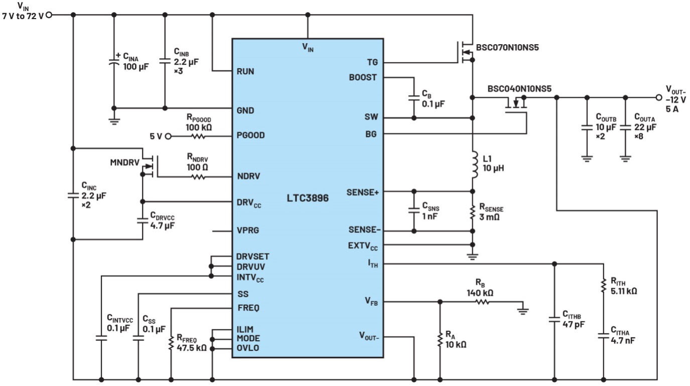
Figure 8. LTC3896 circuit with VIN = 7 V to 72 V, VOUT- = -12 V and fSW = 300 kHz.
Validation of our inductance selection with LTspice.
Regarding the coil current ripple, more accurate values can be obtained by simulating the same LTC3896 circuit with LTspice, as shown in Figure 9. In Figure 10, ΔIL is approximately 1.45 A and 3.5 A, respectively, at VIN = 7 V and 72 V, which is consistent with the first-order approximation values previously extracted using Figure 7 and the scaling of fSW and L. Note that the coil current probeed in Figure 10 is considered positive when flowing towards RSENSE.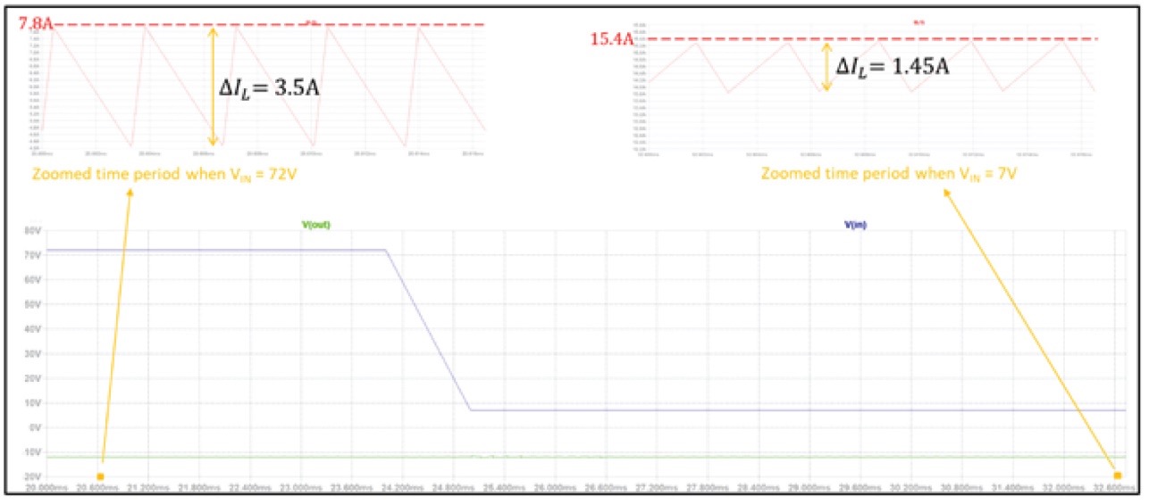
An additional advantage of the LTspice simulation is the ability to determine the peak coil current encountered during operation, which is obtained with the lowest input voltage of 7 V. As shown in Figure 10, our application will face a peak coil current of approximately 15.4 A. Knowing this value allows for the selection of a power inductor with a sufficiently high current rating.
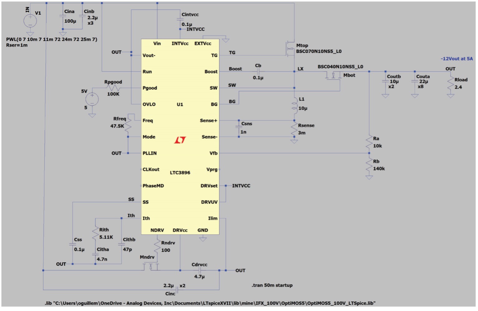
Figure 9. LTC3896 circuit simulated with LTspice.
ΔIL at VIN = 7 V and 72 V and extraction of the coil current peak with the LTspice circuit above.
Design with Even Higher Output Voltages.
Returning to Figure 7, current ripple values were also provided for a hypothetical case with a VIN range of 12 V to 40 V and a VOUT of -150 V.
The first observation is that the current ripple is significantly higher for a higher VOUT while maintaining the same fSW and L. Such a high ΔIL is usually unacceptable, so we would have to apply a larger scaling factor than in the previous example, which means a higher inductance for the same fSW.
The second observation concerns the variation of ΔIL across the entire input voltage range. For the previous example with VOUT = -12 V, ΔIL only increased by about 2.33 from the lowest to the highest ripple value as the input voltage increased more than tenfold. In the current case with VOUT = -150 V, ΔIL already increases by 2.85 from the lowest to the highest current ripple, even though the input voltage only increases by a factor of 3.33 from 12 V to 40 V.
Fortunately, these challenges only exist in CCM. In discontinuous conduction mode (DCM), limitations such as 30% to 70% of IOUT(MAX) no longer apply. In any case, it would be too demanding to convert VIN = 12 V to VOUT = -150 V at IOUT(MAX) = 5 A in a single step. In any case, when such voltage conversions are required, the output current requirement is generally low, which means we are operating in DCM. This is the case, for example, with the circuit on the last page of the LTC3863 datasheet, reproduced in Figure 11.
Due to the low DC currents, using a non-synchronous driver like the LTC3863 was sufficient to provide acceptable efficiency under these conditions. In the case of this LTC3863 design in DCM, the LTC3863 circuit provided with LTspice is a useful tool for optimizing coil selection.
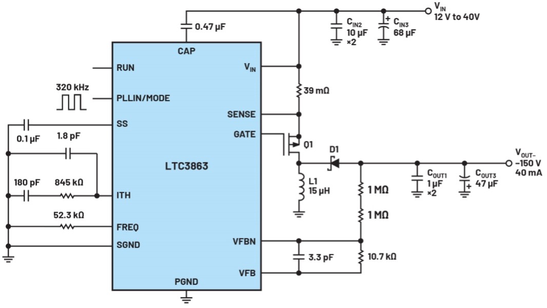
Figure 11. LTC3863 circuit with VIN = 12 V to 40 V, VOUT- = -150 V and fSW = 320 kHz.
Conclusion:
The hot loop of the inverting buck-boost topology includes components located on both the input and output sides, making its design more difficult to implement than that of buck and boost topologies.
Although there are some analogies with boost, the inverting buck-boost faces much greater current ripple under similar application conditions, since its inductor is the only source of power at the output (if we ignore the output capacitance).
For inverting buck-boost applications with high input and/or output voltages, the inductor current ripple is potentially even greater. To contain it, higher inductance values are used compared to the boost topology. A practical example has been used to demonstrate how to quickly scale the inductance based on application conditions.
Reference
1Dostal, Frederik. "The art of generating negative voltages". Power Systems Design, January 2016.
About the author:
Olivier Guillemant is a core applications engineer at Analog Devices in Munich, Germany. He provides design support for the Power by Linear™ portfolio for broad-market European customers. He has held various power applications roles since 2000 and joined ADI in 2021. He earned his master's degree in electronics and telecommunications from the University of Lille, France.